Solving the filter on paper: svf.h
The user-facing chapter promised that tap.svf~ is "unconditionally stable
under per-sample cutoff modulation" and that its morph corners are
"bit-identical to the discrete modes." Promises like that are either
mathematical facts or marketing. This appendix does the math: it derives the
filter the way the file was actually designed, then walks the engineering
decisions that don't show up in a Bode plot — and why each one beat its
alternative.
The reference is Andy Simper's Cytomic technical papers ("Solving the
continuous SVF equations using trapezoidal integration and equivalent
currents"), specifically the SvfLinearTrapOptimised2 form. What follows is
the same derivation with the file's variable names.
The analog prototype, and where digital versions go wrong
The state-variable filter is two integrators in a loop. With cutoff ω and damping k = 1/Q, the continuous equations are:
v1' = ω · (v0 − k·v1 − v2)     (band state: input minus damping minus low state)
v2' = ω · v1                   (low state: integral of band)
Lowpass is v2, bandpass v1, highpass v0 − k·v1 − v2 — every response lives in the same two states, which is what makes an output mix (and therefore a morph) possible at all.
The textbook digital version (Chamberlin) discretizes with explicit Euler: each integrator uses the previous sample's value. That inserts a unit delay into the loop, and a delay in a feedback loop is a stability bomb with a frequency fuse: the design blows up as fc approaches fs/6, and modulating the cutoff re-lights the fuse every sample. The classic workarounds (oversample it, clamp it) treat symptoms.
Trapezoidal integration, and the algebraic loop
The fix is to integrate with the trapezoidal rule — average the old and new derivative — which in filter terms is the bilinear transform. Define the prewarped gain the file computes once per cutoff change:
g = tan(π · fc / fs)
(The tan is the prewarp: it makes the digital filter's response at fc exactly match the analog prototype's, all the way to Nyquist. This single line is why self-oscillation later measures 999.7 Hz for a 1 kHz setting rather than drifting flat.)
Trapezoidal integration of state s with input x is s_new = s + g·(x_old + x_new). Grouping the "old" terms into a memory variable — Simper's equivalent current ic = s + g·x_old — each integrator becomes:
s_new = ic + g · x_new with ic updated as ic_new = 2·s_new − ic
But notice the trap: x_new for the first integrator is the new band value, which depends on the new low value, which depends on the new band value. The new sample appears on both sides — an algebraic loop, exactly the "zero-delay feedback" the initials ZDF refer to. Instead of breaking the loop with a delay (Chamberlin's sin), we solve it. It is linear, so substitution gives a closed form. With v0 the input and ic1, ic2 the two equivalent currents:
v1 = a1 · ic1 + a2 · (v0 − ic2)          the band state, solved
v2 = ic2 + g · v1                        the low state, then follows
where  a1 = 1 / (1 + g·(g + k)),  a2 = g · a1
Those are precisely the file's per-section solve constants (a1, a2, a3 = g·a2 caches the product used by the low state), and the state update is the
canonical TPT pair ic1 = 2·v1 − ic1, ic2 = 2·v2 − ic2.
Why this is unconditionally stable, even modulated: the trapezoidal rule is A-stable — it maps the entire left half of the s-plane (every stable analog filter) inside the unit circle, for any g > 0. Change g every sample and each sample still computes a passive, energy-consistent step; there is no regime of fc or modulation rate where the update gains exceed unity. The notebook's 90 Hz-LFO-through-five-octaves torture test isn't surviving by margin; it's surviving by theorem.
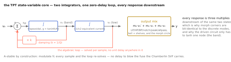
The loop the algebra just solved, and the mixer the next section explains.
The output mix, and why morph corners cost nothing
Every response is a weighted sum over the same solved values:
y = m0·v0 + m1·v1 + m2·v2

lowpass   m = (0,  0, 1)        notch     m = (1, −k, 0)
bandpass  m = (0,  1, 0)        peak      m = (1, −k, −2)
highpass  m = (1, −k, −1)       allpass   m = (1, −2k, 0)
mode_morph linearly interpolates the mix vector around the circle LP → BP →
HP → notch → LP. Two facts follow by construction, not by tuning:
- At a corner, the interpolated vector equals the discrete mode's vector exactly — same floats, same states, same arithmetic. The notebook's measured max difference of 0 is not a tight tolerance; it is an identity.
- Morphing is free. The states don't know the mix exists; sweeping it can never destabilize anything, because it is three multiplies downstream of the filter.
The parametric-EQ trio (bell, shelves) is the same machinery with mix weights that depend on a gain factor A = 10^(dB/40), straight from Simper's tables — and it always runs a single section, because cascading an EQ stage squares its boost: two +12 dB bells are a +24 dB bell, which is never what the user typed.
The cascade: Butterworth spread, resonance on the last section
Orders 4 and 8 run two and four sections at the same cutoff. Stacking identical Q = 0.707 sections would droop the passband (each contributes its −3 dB early); instead the sections take the Butterworth Q spread — the Qs whose product of section responses is maximally flat:
Q_i = 1 / (2·cos θ_i),  θ_i the Butterworth pole angles
order 4: 0.5412, 1.3066        order 8: 0.5098, 0.6013, 0.9000, 2.5629
That is why the measured response sits at −3.01 dB at fc at every order. User resonance then sharpens only the final (highest-Q) section, via
Q_res = Q_base / (1 − r), r ∈ [0, 1) (clamped at 1 − 10⁻⁴)
— one clean resonant peak riding a flat passband, rather than four peaks
compounding. The inverse mapping (resonance_from_q) exists so the wrapper's
q message round-trips exactly.
The driven circuit: one saturation, one pass
The driven circuit places tanh on the band node — in the damping path, where an OTA's transconductance actually compresses. That placement is the whole design: as amplitude grows, the effective damping k·tanh(v1)/v1 grows with it, which is an automatic gain control wrapped around the resonance. Push the loop gain slightly past the oscillation threshold at resonance 1.0 and the filter must oscillate (the linear model's poles are outside the circle) but cannot run away (the saturation restores effective damping as amplitude rises). Bounded self-oscillation is not a limiter bolted on; it is the fixed point of that tug-of-war. An all-zero state solves the equations too — hence "give it a ping."
Solving a nonlinear zero-delay loop exactly needs iteration. The file uses
the one-pass scheme shared with tap.ladder~'s solver_fast: solve the
linear ZDF prediction for the band node, saturate it, commit. The error of
that shortcut is second-order in how much tanh bends over one oversampled
step — and the driven circuit always runs oversampled (2× default), with
4th-order Butterworth anti-image/anti-alias biquad pairs on the way up and
down. At these rates the one-pass and iterated answers are audibly identical;
the ladder file, which drives its nonlinearity much harder, is the one that
also ships a Newton option.
The engineering ledger
Decisions visible only in the code, with their reasons:
- Two-tier coefficient update. Recomputing everything per sample costs a
tan()plus the mix logic even when nothing changed. The file splits state: a shape tier (damping, mix weights, EQ gains — dirtied only when a non-frequency parameter or mode changes) and a cutoff tier (tan and the three solve constants — recomputed only when the incoming cutoff differs from the cached one). Signal-rate modulation pays for exactly what it moves. The benchmark ratchet recorded the win: modulated 2nd-order lowpass 36 → 19 ns/sample, modulated morph 77 → 28, bit-identical output (the morph-corner identity tests pin that "bit-identical" is literal). ramp_todoesn't dirty the shape tier for frequency — the cutoff cache catches it. One branch, measurable at audio rates.- Multichannel by frame protocol. Coefficients are computed once per
tick()and shared by every channel'sprocess(ch, x)— an N-channel engine outside Max for the cost of one solve. The Max wrapper stays mono by house rule (mc.wraps it). - Allocation discipline. The only allocation is the per-channel state
vector in
prepare(); setters are wait-free and safe from the message thread while audio runs, because a "set" is a ramp target plus a dirty flag. - Anti-denormal guard on the states (the
tap.comb~idiom): a filter ringing out into silence otherwise wanders into denormal territory and multiplies its own CPU cost right when the music is quietest. - What is deliberately absent: fast-tanh approximations and a polyphase halfband resampler are both flagged in the file as candidates — and parked, because each changes output microscopically and the project's rule is that optimizations land only bit-identical or explicitly signed off.
Checkpoint
Trapezoidal integration turns the SVF's two integrators into a solvable linear system per sample — A-stability is where the modulation-proofness comes from, prewarping is where the tuning accuracy comes from, and the output mix is where morphing comes from, corner-exact by construction. Butterworth spread keeps cascades flat; resonance sharpens one section; the driven circuit's tanh placement makes bounded self-oscillation a fixed point rather than a feature. The rest is bookkeeping — and the bookkeeping was benchmarked.