Introduction
Space is the place.
— Sun Ra
Close your eyes anywhere — a kitchen, a train platform, a forest — and you still know where everything is. The kettle is behind you and to the left. The announcement echoes from above. Somebody's footsteps approach from the right and pass behind your head. You perform this feat constantly, effortlessly, with two ears and no visible antennas, and almost every recording you have ever made throws that entire dimension away and hands your listener a flat pane of glass: left, right, and a line between them.
This book is about getting the dimension back. It is a field guide to spatial audio — the family of techniques for capturing, composing, and delivering sound that has direction and space — written for people who make sound and have never touched any of it. Its center of gravity is Ambisonics: a sixty-year-old idea, born in British hi-fi research and resurrected by VR, that has quietly become the common language of full-sphere audio. If you have seen the word and nodded past it, or been told "just use fourth order, obviously" by someone who didn't explain, this book is for you.
Who this is for
You are comfortable in Max — you can build a patch, you know what dac~
does, mc. cables don't scare you (and if they do, they will stop within a
chapter). You own a pair of headphones. That is the whole entry requirement.
You do not need: a loudspeaker array, an ambisonic microphone, a degree involving spherical trigonometry, or any C++. There is real mathematics underneath this field, and the book will always tell you where it lives, but the main text works in pictures, listening experiments, and patches. The formulas appear in clearly marked for the curious sidebars you can skip without losing the thread, and the appendix points to the open-access literature when you want the full derivations.
What a "field guide" means
Spatial audio is a territory, not a technique. It contains at least three competing paradigms (channel-based, object-based, scene-based), a zoo of formats (5.1, 7.1.4, Atmos, AmbiX, FuMa, binaural…), and toolchains that span DAWs, visual programming, game engines, and dedicated hardware. People get lost here not because any one idea is hard but because nobody handed them a map.
So this book behaves like a field guide: it teaches you to identify what you're looking at, and it is opinionated about which tool to reach for in which situation — including the situations where the honest answer is "not Ambisonics." Part V distills that judgment into an explicit decision guide; everything before it earns the distillation.
The playground
You learn a territory by walking it. Our vehicle is
AmbiTap, an open-source
higher-order-ambisonics library, through its
Max package: seventeen ambitap.*~
objects that encode, rotate, decode, binauralize, add distance and rooms,
and let you watch a soundfield while you listen to it. Every hands-on
chapter is built around a patch you can open and hear in minutes.
The vehicle is not the territory, though. The same objects exist for Pure Data, and Part IV walks the wider world: ambisonic microphones, the Reaper plugin ecosystem (IEM, SPARTA, ATK, Envelop), game engines and XR middleware, and how all of this relates to Dolby Atmos. The concepts you learn in Max transfer whole; only the object names change.
How this book stays honest
Tutorials rot. Prose describes a patch that no longer matches the software; a hand-drawn diagram flatters a decoder that never behaved that way. This book borrows three mechanical commitments from its sibling (the SampleRateTap book) to resist that:
- Every hands-on chapter opens a real patch. The companion patches ship
inside the AmbiTap-Max package, under
patchers/booklet/. The book never describes a patch that doesn't exist in the repository next to the objects it uses. - Every plot of computed data is generated, not drawn. The figures in
book/src/img/are produced byscripts/generate_book_figures.pyin the AmbiTap repository, which drives the actual C++ library through its C ABI — the same code path the shipping objects run. The ITD curves in Chapter 1 come from the same embedded KEMAR head yourbinaural~object uses. (Purely schematic diagrams — box-and-arrow pictures — are hand-authored SVG and contain no data to lie about.) - Ecosystem claims carry dates. Chapters about plugins, engines, and delivery formats describe a moving landscape; they name versions and say "as of 2026" out loud, so you know exactly what to re-verify later.
The route
- Part 0 — The flat picture. How your ears actually localize sound, why stereo is a narrow trick, and the three paradigms of spatial audio. No tools yet; this is the map legend.
- Part I — First sounds. Headphones on: a source orbits your head within fifteen minutes, you rotate the world, and you send a scene to real loudspeakers. Experience before theory.
- Part II — What's in the bus. What those
(order+1)²channels are, why order controls sharpness, and the format paperwork (AmbiX vs FuMa) that makes files from different decades interoperable. - Part III — The craft, task by task. Each chapter is a thing you want to do: place sources, add distance, build rooms, decode to speaker arrays, go deep on binaural, monitor a scene you can't see, mix inside it, cancel crosstalk, and fold channel-based beds in.
- Part IV — The wider world. Pd, microphones, DAWs, game engines, Atmos.
- Part V — Which tool, when. The decision guide.
What you need
- Max 9 (the objects need Max's multichannel
mc.signals; the optional UI widgets usev8ui). The AmbiTap-Max package, built or downloaded — Chapter 3 covers installation. - Headphones. Closed or open, cheap or fancy — but headphones, not laptop speakers, for every binaural experiment.
- Optional, later: four or more loudspeakers (Chapter 5 onward), Pure Data ≥ 0.54, Reaper (Part IV).
Status of this draft
This is a complete first draft — all parts and appendices are written, the companion patches ship in the packages, and every computed figure regenerates from the library with its claims asserted at build time. What it has not yet had is readers; found something wrong, unclear, or missing, file an issue on the repository like you would for any other bug.
Two ears, infinite directions
Before you buy a single plugin or patch a single object, notice what you already own: the most sophisticated spatial audio system ever built. Two pressure sensors, one head between them, and a brain that turns their tiny disagreements into a continuous, three-dimensional map of everything sounding around you.
Every technique in this book — ambisonic encoding, decoder matrices, HRTF convolution, crosstalk cancellation — is in the business of manufacturing the input signals that system expects. So the right place to start is not with Ambisonics at all. It's with the question the rest of the book keeps answering: what do your ears actually measure?
The three measurements
Your auditory system localizes sound with three families of cues, and it helps to know all three by name, because every spatial audio tool is a machine for forging some subset of them.
Time. (ITD — interaural time difference.) A sound from your left reaches your left ear first. The head is roughly 17 cm wide, sound covers that in about half a millisecond, so the arrival-time difference between your ears ranges from zero (dead ahead or behind) to roughly 0.6–0.7 ms (hard left or right). Half a millisecond is nothing — a single video frame lasts sixty times longer — yet your brainstem resolves differences of ten microseconds. ITD dominates localization at low frequencies, below about 1.5 kHz, where the wavelength is long enough for timing comparisons between the ears to be unambiguous.
Level. (ILD — interaural level difference.) Your head is an obstacle. At high frequencies — wavelengths small compared to the head — it casts an acoustic shadow, so a sound from the left arrives at the right ear not just later but quieter, by up to 20 dB and more in the top octaves. At low frequencies the wave diffracts around the head almost unbothered and the level difference nearly vanishes. This division of labor — timing below ~1.5 kHz, shadow above — is the duplex theory, and it's over a century old.
Spectrum. Time and level differences share a blind spot: they're (nearly) identical for every point on a cone extending sideways from your ear — the cone of confusion. A source directly ahead, directly behind, and directly above can produce almost the same ITD and ILD (all ≈ zero). What breaks the tie is your outer ear. The pinna's folds reflect and resonate differently depending on the direction of arrival, notching and boosting the spectrum above ~4 kHz in a direction-dependent pattern your brain has spent your whole life learning. Elevation perception and front/back discrimination live almost entirely in these spectral fingerprints — which is why they're fragile, personal, and the hardest thing for any playback system to reproduce.
The figure below shows the first two cues, measured, not sketched: the interaural time and level differences of the KEMAR mannequin head — the standard measurement dummy whose ears this book's binaural renderer uses — as a source circles the horizontal plane.
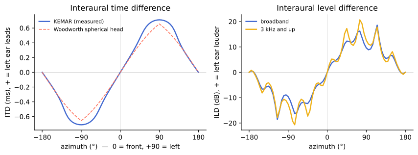
Two things worth noticing. The ITD curve is smooth, bounded, and maxes out around ±0.7 ms exactly as head geometry predicts. The ILD curve is larger, lumpier, and frequency-dependent — that's diffraction around an actual head, with actual ears attached, and its lumps are information, not noise.
For the curious. The duplex theory is Lord Rayleigh (1907); the modern, encyclopedic treatment of everything in this chapter is Blauert's Spatial Hearing. A convenient geometric approximation for ITD is Woodworth's formula, ITD ≈ (a/c)(θ + sin θ) for head radius a and sound speed c — the library's test notebooks check the embedded KEMAR data against it, and you can rerun that check yourself (
notebooks/hrtf_analysis.ipynbin the AmbiTap repository).
And one more cue that isn't a cue: movement. When time, level, and spectrum still leave ambiguity, you turn your head — a few degrees is enough — and watch how the cues change. Front/back confusions collapse instantly. Keep this in your pocket: it is the entire reason head tracking matters, and the reason Chapter 4 exists.
The experiment stereo fails
You don't need any of this book's tools yet. Build the classic MSP patch — a noise burst panned between two speakers or headphone channels:
[noise~] → [pan2 ...] → [dac~ 1 2] (any equal-power pan will do)
Sweep the pan and listen. Something does move. Now interrogate it:
- Where is "behind you"? Try to pan the noise behind your head. There is no knob for that. The image lives on a line between the speakers (or, on headphones, on a line through your skull — more on that in a moment).
- Where is "up"? Same problem. One axis was never captured.
- If you're on loudspeakers: move. Stand up, step a meter to the left, sweep the pan again. The image warps toward the nearer speaker and, from close enough to either one, collapses into it entirely.
What stereo panning actually is
Stereo panning is one trick performed well: play the same signal from two loudspeakers at different levels, and a listener seated exactly on the centerline hears a single phantom image somewhere between them. The pan pot moves the image by trading level between the channels — usually along an equal-power law so the loudness stays constant as it moves:
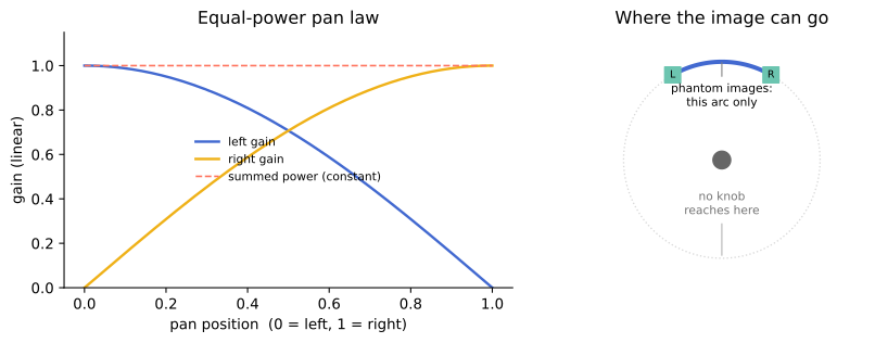
It's worth being precise about why this works, because the mechanism is sneakier than "the louder side wins." Both speakers reach both of your ears. At low frequencies, the two arrivals sum at each eardrum, and the level imbalance between the speakers converts into a timing shift of the summed waveform — fake ITD, synthesized out of pure level difference. The trick is genuinely clever. It is also narrow:
- It only works between the speakers — a ±30° window in front of you.
- It only works at one listening position. Off the centerline, the nearer speaker's earlier arrival dominates (precedence), and the image slides into it.
- It produces no elevation cues and no rear cues — nothing touches the pinna-spectrum channel, and nothing can place energy behind you.
- On headphones, with no crosstalk between channels at all, the level trick stops producing spatial impressions of an external world: images form on the axis between your ears, inside your head. Externalization — the difference between "sound to my left" and "sound in my left ear" — requires the full cue set, which plain level panning never forges.
None of this is a defect. Stereo is a 1930s-vintage compression scheme for space, brilliant within its window, and a century of great records testifies to it. But see it for what it is: a picture of a soundfield, painted on a narrow strip of wall, for a viewer nailed to one spot on the floor.
The point
Localization runs on ITD, ILD, and spectral cues — plus head movement to resolve ties. Stereo forges a sliver of that cue-space. Everything that follows in this book is a machine for forging more of it, more honestly:
- Ambisonic decoding (Chapters 5, 12) arranges many loudspeakers so the cues reconstruct over a listening area instead of a point.
- Binaural rendering (Chapters 3, 13) synthesizes the exact ear-entrance signals — all three cue families — for headphones.
- Head tracking (Chapters 4, 13) keeps the cues consistent when you move, which is the difference between a picture of space and a place.
- Crosstalk cancellation (Chapter 16) fights the physics of two speakers to deliver binaural signals through the air.
First, though, we need a language for storing a soundfield so that any of those machines can render it. That language question — and its three very different answers — is the next chapter.
Three ways to put sound in space
Chapter 1 ended on a question: how do you store a soundfield? Not "how do you play one back" — store one, mix one, send one to a stranger whose playback system you know nothing about?
Every spatial audio format ever shipped answers that question in one of three ways. Learn the three answers and the entire landscape — Atmos, AmbiX, 7.1.4, VBAP, binaural stems, game-engine audio — snaps into a tidy map. This chapter is that map. It contains no patches and no math; it is the most important chapter in the book.
Answer 1: store the speaker feeds (channel-based)
The oldest answer: decide the loudspeaker layout first, then store one audio channel per loudspeaker. Stereo works this way. So do 5.1, 7.1, and 7.1.4: the ".1" file layouts where each channel is, by definition, what comes out of that speaker.
The mix is the render. When you pan a sound "half into the left surround," you are writing signal onto the left-surround channel, and that decision is baked at mix time, forever.
- Strengths. Dead simple. Zero playback intelligence needed — wire channel 3 to the center speaker and you're done. Decades of tooling, room standards (ITU-R BS.775), and engineering craft. Total artistic control over exactly what each speaker emits.
- Costs. The mix assumes that layout. Played on anything else, it must be re-rendered by ad-hoc up/downmix rules ("fold the surrounds into the fronts at −3 dB…"), which are lossy and nobody's favorite. There is no listener rotation — the sound is nailed to the speakers. And channel count scales linearly with spatial resolution: wanting height means shipping four more channels.
Names you'll hear: stereo, quad, 5.1, 7.1, 7.1.4, 22.2, "beds" (a term
from Atmos workflows for a channel-based base layer — Chapter 17 folds
these into ambisonic scenes with ambitap.bed2hoa~).
Answer 2: store the sounds and where they go (object-based)
The second answer refuses to commit to speakers at all. Store each sound as a mono (or stereo) object — the dry audio — plus a metadata track: "at t=12.3 s, this object is at azimuth 40°, elevation 10°, two meters out." At playback time, a renderer reads the metadata and computes, for whatever loudspeakers or headphones actually exist, how to place each object there.
This is how Dolby Atmos delivers height without shipping a channel per speaker, and it is how every game engine has worked since the 1990s: a game can't know your speaker setup, and its sounds move because the world moves, so rendering must happen at playback, per listener, per frame.
- Strengths. Layout-independent by construction — the same master plays on a soundbar, 7.1.4, or headphones, each rendered natively. Individual sources stay discrete and editable to the end: a renderer can place one helicopter with pinpoint precision on whatever speakers are closest. Interactivity falls out for free — move the metadata, the sound moves.
- Costs. The renderer is a black box you don't control; your mix's spatial character is partly its aesthetic decision (ask anyone who has compared the same Atmos master across renderers). Complexity lives in the pipeline: authoring tools, metadata formats, licensing. Object count is a budget — each one is a live audio stream plus math at playback. And a diffuse thing (rain, a crowd, reverb everywhere) is an awkward fit for a format whose atom is "a sound at a point."
Names you'll hear: Dolby Atmos, MPEG-H, ADM/BW64, game-engine "emitters," VBAP (vector-base amplitude panning — the workhorse algorithm object renderers use to place a point source on the nearest speakers; AmbiTap's decoder uses it internally, and Chapter 12 will point at it).
Answer 3: store the field itself (scene-based — this is Ambisonics)
The third answer is the strange one, and the one this book is about.
Don't store speaker feeds. Don't store a list of sources either. Instead, describe the acoustic field at one point in space — the point where the listener's head goes — as a set of signals that together capture sound arriving from every direction at once. Not "channel = speaker," not "track = source," but "channel = a component of the directional field," the way an image file's channels are color components rather than a list of the objects photographed.
That set of signals is called B-format, and the scheme is Ambisonics (Michael Gerzon and colleagues, early 1970s). The first channel (called W) is what an omnidirectional microphone at the listening point would hear — sound from everywhere, no direction. The next three (Y, Z, X) are what three figure-8 microphones at the same point would hear, aimed left–right, up–down, and front–back. Four channels, and the full sphere — behind, above, below — is already represented. That's first-order Ambisonics. Want sharper directional detail? Add channels that capture finer directional patterns: 9 channels for second order, 16 for third, 25 for fourth — higher-order Ambisonics (HOA), and the blur shrinks with each step. (Part II makes this precise; for now, "more channels = sharper picture" is exactly the right intuition.)
The consequences are the point:
- The scene is finished, yet the speakers are not chosen. A decoder — a small matrix, computed once for your actual layout — turns the same B-format scene into feeds for a quad rig, a 30-speaker dome, stereo, or (via virtual speakers and HRTFs) headphones. Mix once, decode anywhere.
- The whole scene rotates for the cost of a matrix. Because the channels form a mathematically tidy directional basis, rotating everything you hear — a hundred sources, the reverb, the recorded crowd — is one small matrix multiply, identical in cost for one source or a thousand. This is why VR standardized on Ambisonics for ambience: head tracking must rotate the world sixty times a second, cheaply. (Chapter 4 puts this under your fingers.)
- Diffuse and discrete coexist. A field description doesn't care whether the energy came from one trumpet or rain on a roof. The awkward case for object formats is the natural case here.
- It's how you record space. An ambisonic microphone (Chapter 19) captures B-format directly. There is no such thing as an "object-based microphone."
- The costs are real too. Sources blur together into the field — you
can't reach in afterward and grab one trumpet the way an object format
can (Chapter 15's
vmic~gets you partway, at the field's resolution). Sharpness costs channel count quadratically. And low orders are genuinely soft-focus: first-order sounds spacious, not pinpoint.
Names you'll hear: Ambisonics, B-format, HOA, AmbiX and FuMa (two conventions for channel order/scaling — the "paperwork" of Chapter 8), ACN/SN3D (the AmbiX conventions AmbiTap uses throughout), "360 audio" (YouTube's spatial audio is first-order AmbiX).
One table
| Channel-based | Object-based | Scene-based (Ambisonics) | |
|---|---|---|---|
| What travels | one signal per speaker | dry sources + position metadata | directional field components |
| Spatial decisions made | at mix time | at playback (renderer) | at mix time (scene), decoded at playback |
| Plays on other layouts | via lossy up/downmix | natively, per renderer | natively, via decoder matrix |
| Rotate the whole scene | no | re-render every object | one matrix multiply |
| Discrete source precision | high (on the reference layout) | highest | limited by order |
| Diffuse material (rain, reverb, crowds) | fine | awkward | natural |
| Capture with a microphone | per-layout arrays | — | directly (ambisonic mics) |
| Cost axis | channels = speakers | objects × renderer math | channels = (order+1)² |
| Flag-bearers | 5.1 / 7.1.4 | Atmos, MPEG-H, game engines | AmbiX, VR/360, research & art |
A photography analogy that will carry us surprisingly far: channel-based is a print, sized for one wall; object-based is the layered project file, re-composited for every screen; scene-based is a panoramic negative — everything that arrived at the lens, developable for any display, but you can no longer un-photograph one pedestrian from the crowd.
So when is Ambisonics the right tool?
The full decision guide is Part V, after you've actually used everything. But the shape of the answer fits in four lines, and you should carry it from the start:
Reach for Ambisonics when the scene is the deliverable: immersive recording, VR/360 ambience, head-tracked anything, music and installations for speaker arrays that vary venue to venue, diffuse and enveloping material, or whenever "mix once, decode anywhere" describes your problem.
Reach for something else when the speakers are the deliverable (a
club PA, a fixed cinema stem — channel-based), when a commercial platform
is the deliverable (a Dolby Atmos release — object-based, because the spec
says so), or when you have a handful of point sources on headphones only
and maximum sharpness matters — direct binaural panning of each source
(Chapter 9's panbin~) beats routing them through a blurring field.
Mixed answers are common and respectable: game engines routinely render foreground objects directly and carry the ambience bed in Ambisonics.
Enough cartography. You now know what Ambisonics is — a stored soundfield — and roughly when to want it. Time to hear one. Headphones on; the next chapter is a patch.
Fifteen minutes to 3D
Theory is over for a while. In this chapter you install the AmbiTap package, build a four-object patch, and hear a sound orbit your head — behind you, above you, all the places Chapter 1 established that stereo cannot go. Then we look at what's flowing through the patch cords, because you will have just used an ambisonic bus without ceremony, and it deserves thirty seconds of admiration.
You need: Max 9, headphones, and about fifteen minutes.
Install the package
Clone and build the Max package (it pulls the AmbiTap library and the
Cycling '74 min-api as git submodules; CMake ≥ 3.24 and a C++20 compiler
required — on macOS that's Xcode's command-line tools):
git clone --recurse-submodules https://github.com/tap/AmbiTap-Max.git
cd AmbiTap-Max
cmake -B build -S . -DCMAKE_BUILD_TYPE=Release
cmake --build build
# externals land in externals/
(If you don't have node/npm installed, add -DAMBITAP_MAX_BUILD_UI=OFF —
it skips the optional UI widgets, which this chapter doesn't use.)
Then let Max see the package — symlink (or copy) the folder into your Packages directory:
ln -s "$PWD" ~/Documents/Max\ 9/Packages/AmbiTap-Max
Restart Max, create a new patcher, and type ambitap.encode~ into an
object box. If it turns into a real object instead of staying amber-broken,
you're installed. (Every object also has a help patch — right-click →
Open Help — which is the package's own reference; this book will lean on
them.)
The patch
Open patchers/booklet/01-first-sounds.maxpat from the package — or
build it yourself; it's small enough to type:
[pink~]
   |
[ambitap.encode~ 3]        ← mono in, ambisonic scene out
   |                          (one thick mc patch cord)
[ambitap.binaural~ 3]      ← scene in, your two ears out
   |    \
[dac~ 1 2]
Four boxes. Note the 3 on both objects — that's the ambisonic order,
and the two must match (the encoder speaks a 16-channel scene at order 3,
and the renderer must expect the same 16 — give both objects the same
number, always). Note also the patch cord between them: it's drawn thicker
than a normal signal cable. That's a Max multichannel (mc.) connection
— one cord, sixteen channels inside it.
Headphones on. Volume low. Start the audio (ezdac~/speaker icon or the
Audio On toggle in the companion patch). You should hear pink noise,
dead ahead, slightly outside your head — already not the
between-the-ears image plain stereo gives on headphones.
Move it
ambitap.encode~ takes an azimuth message — the source's horizontal
angle. One catch, and it's a convention you'll meet across the whole
ambisonics world: angles are in radians, with 0 = front and positive
angles moving left (counterclockwise seen from above, the math world's
habit). Degrees are more comfortable to patch with, so scale them:
[dial]  (range 0–360)
   |
[expr $f1 * 3.14159265 / 180.]
   |
[azimuth $1]
   |
[ambitap.encode~ 3]
Drag the dial slowly and listen: 90° is hard left, 180° is behind you, 270° hard right. Then close your eyes and have the patch do the driving — a slow orbit:
[phasor~ 0.05]                 ← one revolution every 20 seconds
   |
[snapshot~ 30]
   |
[expr $f1 * 6.2831853]
   |
[azimuth $1]
Elevation is the same story: elevation $1, radians, 0 = horizon,
+1.5708 (π/2) = directly overhead, negative = below. Send elevation 0.8
while the orbit runs and the circle tilts up toward the zenith.
Sit with it for a minute. A mono noise source, four object boxes, and you have a sound behind and above you on ordinary headphones. Chapter 1 said elevation and rear placement live in fragile, personal spectral cues — what you're hearing is those cues being forged, in real time, from a measurement of a standard mannequin head (the KEMAR — the same dataset the book's Chapter 1 figure was computed from). Yours differs from the mannequin's, so elevation especially may feel vague or compressed to you; that's expected, it varies person to person, and Chapter 13 is about doing better. Front/back may occasionally flip — you can't turn your head to disambiguate yet. That's Chapter 4.
What just happened
Trace the signal. pink~ is one channel. ambitap.encode~ 3 turned it
into sixteen — hang an mc.scope~ or mc.meter~ on that thick cable
and count. Sixteen copies of the same noise, at sixteen different gains,
and the pattern of gains encodes the direction: this is the scene-based
storage from Chapter 2 made concrete. Wiggle the azimuth dial and watch
the meters redistribute while the sound moves.
Why sixteen? Order 3 → (3+1)² = 16 channels. Order 1 would be 4 channels, order 5 would be 36. What does the order buy? Sharpness. Here is the directional resolving power of a scene at orders 1, 3, and 5 — computed from the library itself, as a polar pattern pointed at your source:
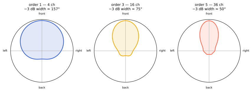
At order 1 the scene knows the sound is "leftish." At order 3 it knows rather precisely. Order 3 at 16 channels is this book's default: sharp enough to be convincing, cheap enough to run stacks of. The full which-order-do-I-need treatment — with the perceptual caveats that make it interesting — is Chapter 7.
ambitap.binaural~ 3 then collapsed the sixteen back to two — but not by
mixing. It rendered the scene to your ears through the HRTF machinery of
Chapter 1: for the field those sixteen channels describe, it computes what
would have arrived at each eardrum, timing, shadow, pinna-notches and all.
Encoder writes the scene; renderer reads it for a device. Everything else
in this book lives between those two boxes.
If something's wrong
- No sound: audio on?
dac~channels 1 2? Max's Options → Audio Status pointing at the right output device? - Sound but no movement: are you actually on headphones? (Laptop
speakers at arm's length turn binaural rendering into mush.) Is the
azimuthmessage reaching the encoder (not the renderer)? - It moves, but in degrees-sized jumps or not at all: check the
radians conversion — a dial feeding
azimuthraw 0–360 sweeps the circle ~57 times. - Stuttering or dropouts: raise Max's I/O vector size to 256+; the binaural convolver is the priciest object in this chapter.
- Different orders on the two objects (say,
encode~ 3intobinaural~ 1): don't. Match them.
Checkpoint
You can now: install the package, encode a mono source into a
16-channel order-3 scene, steer it in azimuth and elevation (in radians),
render the scene binaurally, and see the bus with mc.scope~. One thing
you cannot do yet is turn your head — and that, remember, is how real ears
break ties. Next chapter fixes it with the single most characteristic
ambisonic operation there is.
Turning your head
Chapter 1 left a debt unpaid. Time, level, and spectral cues still leave ambiguities — front/back flips, vague elevation — and real ears settle them by moving: turn your head three degrees and the way the cues change gives the answer away. Chapter 3's orbiting noise couldn't offer you that; however you turned, the scene turned with you, glued to your skull.
This chapter unglues it. Along the way you'll meet the operation that, more than any other, is why Ambisonics exists.
One new box
Open patchers/booklet/02-turning-your-head.maxpat, or splice one
object into Chapter 3's patch:
[pink~]
   |
[ambitap.encode~ 3]
   |
[ambitap.rotate~ 3]        ← NEW: rotates the entire scene
   |
[ambitap.binaural~ 3]
   |    \
[dac~ 1 2]
ambitap.rotate~ takes yaw, pitch, and roll messages — radians
again, so keep the degrees→radians expr idiom from Chapter 3 on a dial.
Park the encoder's source dead ahead (azimuth 0). Now sweep the
rotator's yaw: positive yaw swings the whole scene to your left
(counterclockwise from above, same handedness as azimuth). The source
orbits exactly as if you'd swept the encoder's azimuth — with one source,
you can't tell the difference. So add a second source, because the
difference is the entire point:
[pink~]                [cycle~ 220]
   |                      |
[ambitap.encode~ 3]    [*~ 0.2]
   |                      |
   |                   [ambitap.encode~ 3]   ← azimuth 3.14159 (behind)
   |                      |
   +----------+-----------+
              |
      [ambitap.rotate~ 3]
              |
      [ambitap.binaural~ 3]
Two encoders, their mc cables joined into the rotator's inlet — patch
cords sum, and summing scenes is mixing in ambisonics; the bus doesn't
care how many sources wrote to it. Noise ahead, a quiet tone behind. Sweep
yaw: both move together, rigidly, keeping their 180° separation — the
world turns, not a source. Pitch and roll complete the set: pitch tips
the front of the world down (positive) or up, roll tilts it around your
nose axis.
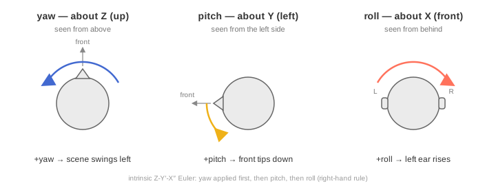
Order of operations (for the curious). The three angles compose in a fixed order — yaw first, then pitch, then roll — as intrinsic Z-Y′-X″ Euler rotations. It only matters when you use two or more at once: yaw-then-pitch and pitch-then-yaw end up in different places. If you ever port a head-tracker driver, this ordering (and the right-hand rule) is the whole game; the library pins it down in
docs/CONCEPTS.md.
Why this box justifies the format
Think about what just happened, in the terms of Chapter 2's three paradigms.
Channel-based: rotating "the mix" is meaningless — the sound is bolted to the speakers. Object-based: rotating the world means visiting every object, every frame, and re-rendering each one; the cost scales with the source count. Scene-based: the rotator never saw your sources. It saw sixteen channels, multiplied them by one 16×16 matrix, and everything in the field — two sources, or two hundred, or a recorded rainstorm with a crowd in it — turned rigidly together. Same cost, always.
That trick is not a bonus feature of the format; it is the format. The channels of an ambisonic scene are components in a directional basis chosen precisely so that rotation is a small, exact, cheap matrix. This is why, when VR needed head-tracked ambience at 60+ updates a second on a phone strapped to a face, the industry reached past its beloved object formats and standardized on Ambisonics for the job.
And it's why the box you just patched is the heart of every VR audio pipeline you've ever heard: head tracking is just yaw/pitch/roll, counter-rotated. If your head turns 30° left, rotate the scene 30° right and the mountain stays put. Any source of orientation data — a phone's gyroscope via OSC, a VR headset, a webcam head-tracker, an IMU taped to your headphones — can drive those three messages. (Sweep the dial smoothly and notice there's no zipper noise: the rotation matrix crossfades in over a few milliseconds, a courtesy you'll learn to expect from every object in the package.)
Two rotators, hiding in plain sight
Here is a subtlety that bites everyone once, so let's get bitten in a
controlled setting. ambitap.binaural~ also accepts yaw, pitch, and
roll. Same words — different meaning:
rotate~yaw turns the world. Positive: the scene swings left past your face.binaural~yaw turns your head. Positive: your virtual head turns left — so a front source now lands at your right ear.
Same axis, opposite visible effect, and both conventions are correct for
what they name. Prove they're inverses with the patch: set rotate~ yaw
and binaural~ yaw to the same value — any value — and the sources snap
back to where they started. World turns left, head turns left with it,
nothing moves relative to your ears.
In practice the division of labor is: scene rotation is composition
(turning the stage, spinning an ambience, choreography — rotate~, mixed
into the scene, heard by every listener) and head rotation is
monitoring (tracking one listener's head — binaural~'s own attributes,
applied at the very end, personal to that render). Part III returns to
this when head tracking gets real hardware attached.
Checkpoint
You can now: rotate an entire scene with one matrix, mix multiple encoded sources onto one bus by joining patch cords, tell world-rotation from head-rotation and cancel one with the other, and explain to a skeptical friend why VR audio runs on Ambisonics. Your scenes still live entirely in headphones, though. Time to put them in a room: loudspeakers next.
Out of the headphones
Binaural rendering is a wonderful lie told to two ears. This chapter tells the truth to a room instead: the same scene you built in Chapters 3–4, decoded to actual loudspeakers, where the soundfield exists in the air and listeners can walk around inside it.
If you don't own four loudspeakers, read on anyway — the chapter ends with what to do about that, and the concepts here (layouts, decoders, channel order) are load-bearing for the whole rest of the book.
The last box
Open patchers/booklet/03-out-of-the-headphones.maxpat, or swap the
renderer at the end of Chapter 4's patch:
[pink~]
   |
[ambitap.encode~ 3]
   |
[ambitap.rotate~ 3]
   |
[ambitap.decode~ 3 quad]      ← scene in, four speaker feeds out
   |
[mc.dac~ 1 2 3 4]
ambitap.decode~ takes two creation arguments: the order (match the
bus, as always) and a layout name that fixes how many output channels
it produces and where it assumes the speakers are. The built-in layouts:
| Layout | Speakers | Where |
|---|---|---|
stereo | 2 | ±30° front pair |
quad | 4 | ±45°, ±135° — a square around you |
hexagon | 6 | a 60°-spaced ring |
octagon | 8 | a 45°-spaced ring |
surround_5_1 | 5 | ITU 5.1 angles (no LFE — see below) |
surround_7_1 | 7 | 7.1 angles (no LFE) |
surround_7_1_4 | 11 | 7.1 plus four height speakers |
cube | 8 | lower + upper square: full 3D |
The decoder's output is one mc cable, one channel per speaker, in the
layout's canonical order — for quad that's front-left, back-left,
back-right, front-right. mc.dac~ 1 2 3 4 then maps those onto your audio
interface's outputs in that order, so the only setup job is knowing which
interface output feeds which physical speaker (and passing mc.dac~ the
right numbers if it isn't 1–4).
Setting up four speakers honestly
The decode assumes a listener at the center of a square of speakers. You don't need an anechoic chamber, but three disciplines repay you instantly:
- Equal distances. The math assumes all speakers equidistant from the center. A tape measure is a spatial audio tool.
- Equal levels. Play pink noise through each speaker in turn (sweep the encoder azimuth to 45°, 135°, −135°, −45° — at those exact angles, a quad decode hands one speaker most of the signal) and match by ear or SPL meter.
- Angles as advertised. ±45° and ±135° from the listening position — the decoder is computing gains for those directions, not for wherever the furniture allowed. Close counts; 20° off doesn't.
Now run the orbit from Chapter 3. Walk around. Sit in the middle and sweep
the rotator's yaw. Notice what headphones couldn't give you: the field is
in the room — externalization for free, no HRTF required — and several
people can hear it at once. Notice also what got worse: away from the
center, images pull toward the nearest speaker (Chapter 1's precedence
effect, back for revenge), and a four-speaker ring has no idea what "above"
means — send elevation 1.0 and the circle just… flattens. Height needs
height speakers (cube, surround_7_1_4) or headphones.
What the decoder actually did
Chapter 2 promised: a decoder is a small matrix computed once for your
layout. Concretely, ambitap.decode~ 3 quad built a 4×16 matrix — four
speakers, sixteen scene channels — and every sample of your speaker feeds
is that matrix applied to the bus. All the intelligence lives in choosing
the matrix; there are competing philosophies, and the object exposes them:
- the
decoder_typeattribute selects the construction —mode_match(the default),allrad, orepad; - the
max_reattribute (off by default) applies a per-order weighting that trades a little theoretical sharpness for cleaner energy concentration — usually a good trade in real rooms.
Chapter 12 is an entire chapter about that choice, with figures computed
from the actual matrices, and a rule of thumb for which construction suits
which array. For a regular ring like quad, the honest summary is: the
defaults are fine, try max_re 1, and don't lose sleep.
One deliberate omission: there is no LFE channel anywhere in this. The
surround_5_1 layout is five full-range speakers. An ambisonic scene
describes direction, and sub-bass direction is barely perceptible —
so LFE/bass management is a playback concern, handled downstream of the
decode (Chapter 17 shows the routing when we meet channel-based beds).
No speakers? Two honest options
Option one: stereo decode. ambitap.decode~ 3 stereo produces feeds
for a normal ±30° speaker pair. It works — the frontal stage is stable and
CPU cost is nil — but understand what it is: a projection of your sphere
onto stereo's narrow window. Rear and height content doesn't vanish (the
decode folds it in at reduced level so energy isn't lost), but it no longer
sounds behind you. It's the right tool for "my ambisonic piece needs a
stereo bounce," not for monitoring spatial decisions.
Option two — the recommended one: keep monitoring binaurally. This
isn't a consolation prize. ambitap.binaural~ is a decode — internally
it renders the scene as if through a fine array of virtual loudspeakers,
each convolved to your ears — and it's a truthful monitor for direction,
which is what you're composing with. Professionals mixing for domes they
visit twice a year work exactly this way: compose binaurally, decode on
site, spend the precious room time on level calibration instead of
composition. The companion patch is wired for the same discipline — the
quad decode and a binaural monitor side by side, one mc gain to switch
between them — so "check it on speakers" stays a five-second habit even
when the speakers are hypothetical.
Checkpoint — and the end of the beginning
You can now take a scene from silence to sound three different ways: binaural for headphones, a quad ring, a stereo fold-down — same scene, one box swapped. That's the "mix once, decode anywhere" promise of Chapter 2, demonstrated rather than asserted.
You also, quietly, now hold the entire ambisonic signal chain: encode → transform → decode. Everything else in this book is a richer version of one of those three stages — fancier sources into the bus (rooms, recordings, beds), fancier transforms on it (mirrors, compressors, virtual microphones), fancier renders out of it (arrays, personalized HRTFs, crosstalk cancellation). Before the craft, though, one debt from Chapter 3 is still outstanding: what are those sixteen channels, actually? Part II opens the bus.
One omni and a lot of figure-8s
Part I left you using a sixteen-channel bus the way you use electricity — gratefully, and without looking inside. This chapter opens the box. There is real mathematics in here (spherical harmonics — the same functions that describe electron orbitals and planetary gravity fields), but you will not need any of it to understand the channels, because every one of them has a physical interpretation you already know from a mic locker:
Every ambisonic channel is a microphone pickup pattern, all of them occupying the same point in space, each aimed differently.
Order 1, channel by channel
Start with the four channels of a first-order scene — classic B-format. Here they are, drawn as polar patterns by the library itself (solid = positive lobe, dashed = polarity-inverted, exactly like the pattern diagrams in a microphone's spec sheet):
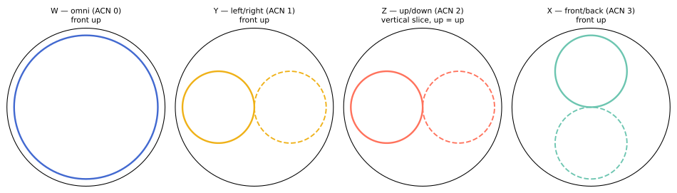
- W is an omni: the sound pressure at the listening point, direction-blind. Every source in the scene is in W at full level, wherever it is. If you keep only W, you have a correct mono mix — worth remembering when a client asks for the mono version.
- Y is a figure-8 aimed left–right: positive lobe left, negative lobe right. A source on the left appears in Y in phase with W; a source on the right appears polarity-flipped; a source dead ahead doesn't appear in Y at all.
- Z is the same figure-8 aimed up–down.
- X is the same figure-8 aimed front–back.
If you have ever set up a mid-side recording — a mid mic plus a sideways figure-8, matrixed into stereo width later — you already own the key intuition: B-format is mid-side, completed. M/S captures "the sound, plus how left-or-right it is." W/X/Y/Z captures "the sound, plus how left-or-right and front-or-back and up-or-down it is." Everything else about Ambisonics is this idea, refined.
Encoding is just gains
Now reread what ambitap.encode~ did in Chapter 3, in these terms. To
place a mono source in a direction, the encoder asks: what would each of
these coincident microphones pick up from a source over there? — and the
answer, per channel, is just a number. A source dead ahead: W gets 1, X
gets 1, Y and Z get 0. A source hard left: W gets 1, Y gets 1, X and Z get
0. A source up-front-left: some spread of positive fractions. Encoding a
source is multiplying one signal by one gain per channel — which you
verified with your own eyes on the mc.meter~ in Chapter 3, watching the
gains redistribute as the dial turned.
That's also why summing two encoded buses (Chapter 4) is legitimate mixing: each channel of the sum is exactly what that virtual microphone would have picked up with both sources playing. The bus doesn't store sources; it stores what the microphones hear, and microphones hear everything at once.
Higher orders: sharper microphones
Four coincident patterns can only distinguish direction so finely — you
felt that as first-order blur in Chapter 3's polar figure. The fix is
more patterns with more lobes. Second order adds five channels whose
shapes are cloverleaf-like, four-lobed patterns; third order adds seven
more, finer still. Each new order family adds 2n+1 channels, which is
why a full set to order N is (N+1)² — 4, 9, 16, 25, 36…
These higher patterns stop resembling anything in a mic catalogue, but their job doesn't change: each is one more coincident pickup pattern, one more independent measurement of the directional field, letting the scene distinguish directions the lower orders confuse. More measurements, sharper picture — precisely quantified in the next chapter.
For the curious. The patterns are the real spherical harmonics Ynm(θ, φ) — the natural basis for functions on a sphere, as sines and cosines are for functions of time. "Order" n is the polar degree; within an order, m runs −n…+n, giving the 2n+1 members. The encoder's gain for channel (n, m) is literally the value of Ynm evaluated at the source direction. The book's figures compute these through the library's
evaluate_sh— which is cross-checked against SciPy, spaudiopy, and pyshtools to float precision (docs/COMPARISON.md) — and Appendix D points to Zotter & Frank's open-access textbook for the derivations.
The two pieces of housekeeping
A basis is only usable if everyone agrees how to file it. Two conventions pin down the bookkeeping, and AmbiTap follows the modern standard (AmbiX) for both:
Channel order — ACN ("Ambisonic Channel Number"). Channels are indexed
acn = n(n+1) + m: W is 0; then Y, Z, X are 1, 2, 3; then the five
second-order channels 4–8, and so on. Note the first-order order: Y
before Z before X — not the historical "XYZ" — a fact that will matter
in Chapter 8, when we meet files that filed things differently.
Level scaling — SN3D. Each pattern needs a reference level. SN3D
scales so that no channel's gain ever exceeds W's: a unit source dead
ahead puts 1.0 in W and 1.0 in X, and anything higher-order lands at 1.0
or below. The practical consequences: your mc.meter~ never shows a
higher channel hotter than W for a single source, and W alone remains a
correctly-scaled mono mix.
You never chose these conventions in Part I, and mixing entirely inside AmbiTap you never need to — every object speaks AmbiX. The moment a file, a plugin, or a 2009 sample library enters the picture, conventions become the difference between a soundfield and soup. That's Chapter 8. First: what does order actually buy, in numbers you can plan a project with?
Order and blur
"Which order do I need?" is the first question every newcomer asks and the question most answers dodge. This chapter answers it with numbers computed from the library, then adds the perceptual caveats that make the honest answer more interesting than the numeric one.
The exchange rate
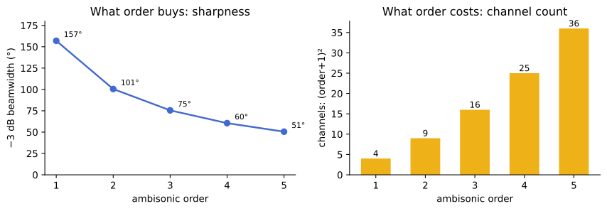
An ambisonic scene at order N resolves direction about as finely as a beam this wide — here is the −3 dB width of the sharpest well-behaved (max-rE) beam the scene can express, against the channel count you pay for it:
Read the two panels together and the economics of the format fall out:
- Order 1 (4 channels): a beam ~157° wide. "Leftish." Genuinely enveloping, genuinely vague. This is what a first-order microphone records and what YouTube 360 plays back.
- Order 3 (16 channels): ~75°. Sources have places, not regions. The workhorse order — sharp enough to compose with, cheap enough to run many of.
- Order 5 (36 channels): ~51°. Noticeably focused; also nine times first-order's channel count, in CPU, disk, and patch-cord width.
Sharpness improves roughly like 1/order, but cost grows like order². Each step up buys less blur reduction than the last and costs more channels than the last — that is why the answer to "which order?" is a judgment call rather than "the biggest number you can afford."
What blur actually sounds like
"Beamwidth" is a proxy. What you hear, order by order, is a bundle of effects — worth knowing individually, because different projects care about different ones:
- Source focus. At low order a point source sounds wide — pleasant for ambience and pads, wrong for a fly buzzing past an ear.
- Separation. Two sources 30° apart are one wide source at order 1, and two events at order 3+. If your material is dense and positional (dialogue scenes, counterpoint spatialization), order buys audible polyphony.
- Sweet-spot size. On loudspeakers, higher order holds the image together over a larger listening area — the low-order image collapses toward the nearest speaker sooner as you move off-center. For installations where people wander, this is often the main reason to pay for order.
- Rear/height solidity on sparse arrays. Where speakers are far apart, low order leans harder on the decoder's interpolation; images between speakers get phasey sooner.
The honest complications
The clean curve above comes with three riders that practitioners learn by expensive experience, offered here at book price.
1 — Your renderer caps what order can deliver. Binaural rendering with a non-individual HRTF (Chapter 3's mannequin ears) blurs elevation and front/back on its own; beyond roughly order 3, extra scene sharpness gets laundered through those borrowed ears and much of it is lost. On headphones with the stock KEMAR set, order 3 versus order 5 is a subtle A/B; on a good 30-speaker dome it is not subtle at all. Match spend to renderer.
2 — Microphones lag encoders. A synthetic scene can be order 5 at the cost of CPU. A recorded scene is bounded by hardware: the ambisonic microphones you can buy run from order 1 (most) through order 4 (Eigenmike em32-class instruments) — Chapter 19 surveys the market. Plan hybrid: recorded first-order bed + encoded higher-order foreground is a respectable, common design.
3 — Order interacts with frequency. The scene reconstructs the field accurately only up to a frequency that rises with order (and shrinks with listening-area radius). Above it, reproduction degrades gracefully from "physically correct" to "psychoacoustically plausible" — which is why decoders apply the max-rE weighting you met as an attribute in Chapter 5: it optimizes the plausible regime that most of the audio band actually lives in.
For the curious. The reconstruction limit is the "kr rule": accurate holography holds roughly while N ≥ kr, with k the wavenumber and r the head/area radius. For a head (r ≈ 8.75 cm) that's about 700 Hz per order — order 3 reconstructs to ~2 kHz, and everything above relies on energy-vector psychoacoustics (hence max-rE, which maximizes exactly that vector). Zotter & Frank ch. 2 (Appendix D) derives all of it. The beamwidth figure and this chapter's numbers regenerate from the library via
scripts/generate_book_figures.py, with the monotonic sharpening asserted at build time.
The planning table
Rules of thumb, not laws — each row assumes the renderer can keep up:
| Order | Ch. | Reach for it when |
|---|---|---|
| 1 | 4 | Recorded ambience beds; YouTube/360 delivery; maximum compatibility; "spacious" beats "precise" |
| 2 | 9 | Tight channel budgets (games, mobile) that still want believable movement |
| 3 | 16 | The default. Composition, installation, VR foreground, binaural work with stock HRTFs |
| 4–5 | 25–36 | Large speaker arrays and domes; wandering audiences; research; personalized-HRTF binaural |
| 6+ | 49+ | Specialist arrays and papers. AmbiTap computes to order 10; your ears in a normal room plateau far earlier |
And a rule of thumb for changing your mind: you can always truncate an ambisonic scene (drop the higher-order channels of an order-5 mix and you have a legitimate order-3, then order-1, mix — the format nests). You can never add order to a recording after the fact. When in doubt, produce one order higher than you plan to deliver.
Order chosen, channels understood — one hazard remains before the craft chapters, and it's the one that bites hardest in the wild: two files can both say "Ambisonics" and disagree about what the channels are.
The paperwork: formats and conventions
Sooner or later — usually the day a collaborator sends "the ambisonic stems" — you will play a B-format file and hear something almost right: levels off, the image smeared, front and left subtly traded. Nothing is broken. You have met the field's history, encoded as channel order.
This chapter is short, practical, and worth its weight in un-smeared mixes.
Two dialects
Ambisonics predates its own standardization by four decades, so there are two families of convention in the wild:
FuMa (Furse–Malham), the historical dialect. First-order channels in
the order W, X, Y, Z, and W recorded 3 dB down (a −3 dB factor,
1/√2, inherited from analog-era headroom practice, with further
per-channel factors at higher orders). Four decades of recordings,
.amb files, classic tools (and the SoundField microphone lineage) speak
FuMa. Defined cleanly only up to order 3.
AmbiX (2011), the modern standard and the only thing new systems
should emit. Channels in ACN order — W, then Y, Z, X (the
n(n+1)+m indexing from Chapter 6) — at SN3D scaling, no W
attenuation. Everything in AmbiTap, every current game engine, YouTube,
and essentially all software written this decade speaks AmbiX.
Same soundfield, two filing systems:
| FuMa | AmbiX (ACN/SN3D) | |
|---|---|---|
| First-order order | W X Y Z | W Y Z X |
| W level | −3 dB (×1/√2) | full scale |
| Higher orders | per-channel legacy factors ("maxN"), defined ≤ order 3 | one rule, any order |
| You'll meet it in | .amb files, older recordings & plugins, SoundField heritage | everything modern; assume it unless told otherwise |
What mismatch sounds like
Feed FuMa into a system expecting AmbiX and two things happen at once. The W attenuation reads as a level/balance error (the omni content 3 dB shy, so the scene sounds oddly hollow and over-directional). The X↔Y swap reads as a geometry error: front-back content lands on the left-right axis and vice versa — the image doesn't rotate so much as fold. It is exactly weird enough to waste an afternoon, because it still sounds "spatial."
The fix is one object:
[ambitap.format~ 3] attribute: direction — fuma_to_ambix / ambix_to_fuma
Multichannel in, multichannel out, orders 0–3 (a FuMa limitation, not an AmbiTap one), exact published conversion factors (they're pinned by exact-value tests in the library, against the AmbiX specification's own tables). Put it at the border the moment anything historical crosses into your patch, and forget it's there.
The rest of the paperwork
Channel order and scaling are the big two; three smaller lines complete the customs form.
Angles and axes. AmbiTap: radians; azimuth 0 = front, positive = counterclockwise from above (+90° = left); elevation positive = up; rotations yaw-then-pitch-then-roll (Chapter 4's figure). Other tools may speak degrees, measure azimuth clockwise, or compose Euler angles in another order. None of this corrupts a file — it corrupts control data, which is why a head-tracker driver is where you'll meet it.
"B-format" is ambiguous on its own. Historically it implied FuMa; today people say it for any ambisonic bus. When a collaborator offers B-format, the professional reply is three questions: what order, what channel order (FuMa or ACN), what normalization (SN3D or N3D)? — that last one because some research tools emit N3D, a cousin scaling in which higher-order channels run hotter than SN3D by fixed per-order factors (√(2n+1); the fix is per-channel gains, and knowing the name is most of the battle).
Files. There is no dedicated ambisonic file format in common use —
scenes travel as ordinary multichannel WAV (or WavPack/FLAC), and the
convention travels as metadata at best, folklore at worst. .amb is a
WAVE variant that reliably means FuMa. A 4- or 16-channel .wav means
whatever its maker meant; a README beats a filename. When you export:
AmbiX, state "AmbiX (ACN/SN3D), order N" in the delivery notes, and
you've done your part for civilization.
For the curious. The AmbiX specification is Nachbar, Zotter, Deleflie & Sontacchi, AMBIX — A Suggested Ambisonics Format (Ambisonics Symposium 2011) — short and readable. The FuMa↔AmbiX factor tables it publishes are the ones
format~implements; the library'sdocs/COMPARISON.mdrecords the exact-value tests, and its ACN⇄FuMa index map is eight integers you can read yourself indsp/format_converter.h.
Checkpoint — and the end of the theory
Part II in three sentences: an ambisonic scene is a set of coincident microphone patterns (order 1: one omni, three figure-8s). More orders mean finer patterns, sharper images, quadratically more channels, and order 3 is the sensible default. Modern channels are filed ACN/SN3D — "AmbiX" — and one object repairs history when it knocks.
That is all the theory this book makes you carry. From here on, every chapter is a job: placing sources, adding distance, building rooms, decoding to arrays, and the rest of the craft. Patch cords from here to the end.
Placing sources
Part III is organized by job, and the first job is the daily one: take
some mono material — synths, samples, stems, live inputs — and place each
piece somewhere deliberate. You already own the mechanics (encode~,
azimuth, elevation, summed buses); this chapter is about doing it well,
at mix scale, and about the one architectural fork the job hides.
Companion patch: patchers/booklet/04-placing-sources.maxpat.
The bus discipline
A workable spatial mix in Max is one habit applied consistently: one
mc. cord is the master scene, every source gets its own
ambitap.encode~ N, and everything sums into that cord before the
renderer. The companion patch lays out three sources this way — noise, a
tone, a click pattern — each with its own azimuth/elevation controls, so
the mix reads like a mixer: channel strips into a bus.
Practical notes that save real time:
- Give every encoder the same order. One order-1 encoder summed into an order-3 bus doesn't crash — its 4 channels land on the first 4 of 16 — and the result is even legitimate (a deliberately blurrier source, the nesting property from Chapter 7). But do it by decision, not by typo; a source that refuses to sharpen is the classic symptom.
- Set levels before the encoder (a
*~per source, or the encoder'sgainattribute — same thing). The bus is a sum; balance is easiest while each voice is still mono. - Automate angles like any parameter. The
azimuth/elevationsetters ramp click-free over a few milliseconds (every AmbiTap parameter does — the library's "click-free contract"), soline,function, LFOs, and live dials are all fair game. For fast circular movement prefer driving azimuth from a phasor (Chapter 3's idiom): it wraps cleanly at ±180° where a naivelineramp would spin the long way round. - Park a monitor on the bus. An
mc.meter~tells you instantly which source just clipped the scene; Chapter 14 upgrades this to real soundfield instruments.
Elevation earns its keep
New spatializers overuse azimuth (the party trick) and underuse elevation (the depth of field). Two placements that transform dense mixes:
- Tilt the pads up. Ambient beds at +30–45° elevation stop competing with foreground material at ear level. The mix gains a vertical layer cake structure that stereo literally cannot express.
- Keep transients near the horizon. Elevation perception (Chapter 1) is spectral and fragile; percussive, broadband material reads its height cues best, but everything localizes most stably at ear level. The horizon is your focal plane.
The fork: through the bus, or around it?
Now the architectural decision this chapter exists to teach. For headphone delivery, there are two ways to render a placed mono source, and the package ships both:
Through the scene: encode~ 3 → bus → binaural~ 3. The source
becomes part of the field, subject to the field's order-3 blur (~75°
beam, Chapter 7), rotatable with the world, mixable with everything else.
Cost: one convolver bank total, however many sources — the renderer
binauralizes the whole bus at once.
Around the scene: ambitap.panbin~ — mono in, azimuth/elevation
messages, stereo out. It convolves this one source directly with a
per-direction HRTF (the full order-5 resolution of the embedded KEMAR
set), skipping the bus entirely. No order-limited blur: this is as sharp
as the dataset gets. Direction changes crossfade click-free. Cost: one
convolution pair per source, and the result is a stereo signal — it
can't be rotated with the scene, vmic~'d, or decoded to a dome; it's
already rendered.
The trade in one line: the bus scales, the direct path sharpens.
encode~ → bus → binaural~ | panbin~ per source | |
|---|---|---|
| Sharpness | order-limited (order 3 ≈ 75° beam) | full HRTF resolution |
| CPU | ~flat with source count | linear per source |
| Rotates with scene / head-trackable via bus | yes | no |
| Decodable to speakers later | yes | no — headphones only |
| Best for | scenes, beds, many sources, anything with a future on speakers | a few precious foreground sources, headphone-final work |
The companion patch wires the same source both ways behind an A/B switch.
Listen at 90° azimuth: through the order-3 bus the source is a presence
to your left; through panbin~ it is a point. Then imagine forty of
them and check the CPU meter. Both instincts are correct; that's why both
objects exist. (Game engines reached the same design decades ago —
Chapter 21 — rendering foreground objects directly and carrying the
ambience in a bus. You are allowed to mix strategies within one patch:
panbin~ the soloist, bus the orchestra, sum the stereo outputs.)
Checkpoint
You can place and automate any number of sources on a disciplined bus, you use elevation as a mixing dimension, and you can argue both sides of bus-versus-direct rendering and pick per source. Placed sources still float in an airless void, though: every source is somewhere, but no source is far away. Distance is its own set of cues, and the next chapter manufactures them.
Distance
Sweep an encoder's azimuth and the source moves convincingly. Now try to make it walk away. There is no knob: azimuth and elevation are angles on a sphere of fixed radius, and nothing in Part I or II ever said how far away that sphere is. Distance isn't a direction — it's a bundle of physical side effects, and to place a source at three meters you manufacture the side effects of three meters.
Companion patch: patchers/booklet/05-distance.maxpat.
What "far" sounds like
Four cues, in rough order of importance:
- Quieter. Level falls as 1/distance (−6 dB per doubling) for a point source in free space — less steep indoors, where walls return energy.
- Duller. Air absorbs high frequencies; a distant source is low-passed by the atmosphere itself. Subtle per meter, decisive per hundred meters.
- More room, less source. At distance, the reverberant field swallows the direct sound; the direct-to-reverb ratio is arguably the strongest distance cue indoors. (This one needs a room to exist — next chapter's job.)
- Late — and shifting when moving. Sound takes ~2.9 ms per meter to arrive. A constant delay is nearly inaudible on its own, but a changing distance turns propagation delay into pitch: the Doppler effect, the single most physical "it's really moving" cue there is.
And one anti-cue for close range: a near source (inside about a meter) gets a bass boost from wavefront curvature — the same physics as microphone proximity effect. Ambisonics has a name for compensating it (NFC, near-field compensation), and it's the difference between "at my shoulder" reading as intimate versus just loud.
One object for the bundle
ambitap.distance~ packages the whole chain for a bus — Doppler delay,
then 1/r gain, then air-absorption low-pass, then per-order NFC shelving
— driven by a single master parameter, in meters:
[ambitap.encode~ 3]        ← direction, as always
    |
[ambitap.distance~ 3]      ← distance 3.5   (meters)
    |
   bus …
The controls that matter, in the order you'll reach for them:
distance— the meters. Automate this and everything downstream follows. Distance changes glide rather than jump: the internal delay slews, which is what makes fast automation produce a genuine Doppler pitch bend instead of a click (the same slewing you can watch measured against 1 ± v/c in the library'sdsp_behaviornotebook).reference_distance— the "zero dB" range: the distance at which the object applies no gain change. Set it to where you balanced the source in Chapter 9's mixing pass (default 1 m), so adding distance processing doesn't re-balance your mix.attenuation— the 1/r exponent. 1.0 is free-field physics; real rooms behave shallower (0.5–0.8), and cinematic taste is often shallower still. This is a style control wearing a physics costume.air_absorption— depth of the high-frequency loss. Physical default; exaggerate for haze, zero it for clinical.doppler/nfc— toggles for the two ends of the chain: Doppler matters when things move fast, NFC when things come close. Both on by default; turn Doppler off for material where pitch is sacred (a distant choir shouldn't detune as it drifts).
Order the chain correctly by instinct: distance~ sits after the
encoder (it operates on the source's bus representation), one per
source-with-a-range; sources that live at a fixed comfortable distance
don't need one at all.
There is also a lone ambitap.doppler~ — just the variable
propagation delay, no gain/air/NFC — for when you want the pitch physics
à la carte (classic use: a synthetic fly-by where you're drawing the
level curve by hand anyway).
The experiment
The companion patch puts a ticking source on the bus with a distance dial spanning 0.3–40 m and each stage on its own toggle. Three things to do with it, ears closed to theory:
- Sweep distance slowly with everything on. Note how little of the effect is level once air absorption joins in past ~10 m.
- Automate a fast pass (2 m → 30 m in two seconds). Toggle
doppleroff and on. Off: a fader move. On: something goes by. - Creep inside 1 m and A/B
nfc. With it, the source leans into your face; without, it's merely near. (Binaural rendering makes this easiest to hear; on speakers, NFC's benefit depends on the array radius — the decode chapter returns to this.)
What you will not get, even with everything on: true "far away" indoors. A source at the end of this chain in a dry scene sounds like a quiet, dull, correct object in an anechoic void — because cue #3, the room, is still missing. That's next.
Checkpoint
Distance is manufactured, not dialed: 1/r, air, delay/Doppler, NFC — one
object chains them per source, with reference_distance protecting your
mix balance and taste controls (attenuation, air_absorption)
adjusting how much physics you want. The void problem remains, and it's
the best possible motivation for the next chapter: rooms.
Rooms
Every scene you've built so far takes place in deep space. Perfectly placed sources, correct distance chains — and no there there, because in real life almost nothing reaches your ears exactly once. The floor, the walls, the ceiling all answer, and that answer is most of what "sounding like a place" means. It's also, on headphones, the strongest lever on externalization: dry binaural sources love to collapse into your skull; give them a floor reflection and they step back outside.
Companion patch: patchers/booklet/06-rooms.maxpat.
What a room does, on a clock
Clap once in a rectangular room and the reply has anatomy — here rendered by the library's own room model (an 8 × 6 × 3.5 m room; every dot is one mirror-image copy of the source):
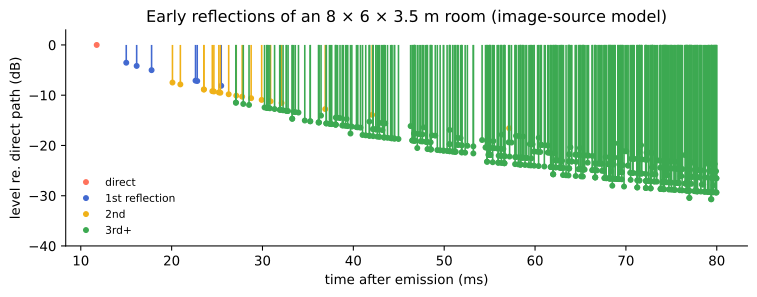
- The direct sound arrives first — alone, and the ear's localization locks onto it (the precedence effect, working for you this time).
- Early reflections follow within tens of milliseconds: first the floor and nearest walls, sparse and loud, each from a definite direction. These carry the room's size and shape — and the source's position in it.
- The tail: reflections of reflections, thickening (the figure's green wall) into a directionless wash whose decay time — RT60, the time to fall 60 dB — is the one number everyone quotes about a room.
A convincing room needs all three, with the right directions on the early part — which is exactly why doing this in ambisonics is special: the reflections are placed on the sphere like any other source, so the room turns with the scene when you rotate, and decodes to any rig.
One object, one room
ambitap.room~ is a mono-in, bus-out room simulator: direct path +
image-source early reflections + a 16-line feedback-delay-network tail,
all SH-domain, all on one HOA cord:
[click~ / your source]
    |
[ambitap.room~ 3]          ← creation arg: order (max 3)
    |
   bus …
You describe the situation, not the effect: dim_x/y/z (the room, in
meters), source_x/y/z, listener_x/y/z (positions in it), and rt60
(seconds). The object derives the reflection pattern from the geometry —
move source_x and the early reflections re-aim themselves, which no
"stereo reverb on a send" can do.
The taste controls:
direct/er/tailtoggles — the anatomy, soloable. The fastest way to learn rooms iseralone while moving the source; the fastest way to mix them istaildown when the wash swallows clarity.gain— the wet level overall.rt60band <hz> <sec>— per-band decay (bright rooms decay treble fast; state it per band rather than faking it with EQ).reflections <6 floats>— per-wall reflection coefficients (deaden the ceiling, liven the floor).absorption fir|iir— quality/CPU switch for the tail's absorption filters:fir(default) is the verified linear-phase set;iiris far cheaper and trades exact mid-band RT60. On a laptop full of rooms,iiris the honest setting.
Two costs to know about, stated plainly because the object won't hide them: the room adds a fixed ~53 ms of latency at 48 kHz (an alignment inherent to the verified design — fine for composition and installation, wrong for monitoring a live input through it), and convolution makes it one of the package's heavier objects — budget rooms like you budget reverbs, not like you budget filters.
Using it like a mixer, not a physicist
- One room, many sources is the normal architecture: sources that
share a space should share a
room~'s tail. The object is mono-in, so the practical pattern for N sources in one room is: give the featured source (or two) its own fully-positionedroom~, and let the rest share one room fed by a mono sum — ears forgive shared early reflections far more than they forgive N different rooms. - Dry/wet is
directversus the rest. The object renders the direct path too, so a source can run entirely through it; or killdirectand treat it as a pure send alongside your Chapter 9/10 chain. - Match the room to the claim. The distance chapter's cue #3 —
direct-to-reverb ratio — now works: a source far away in the room
coordinates automatically gets more room than source. Set the
geometry to agree with your
distance~settings and the illusion compounds; contradict it and ears notice something is off without knowing what. - Design visually when geometry gets fiddly: the package ships
patchers/ambitap.roomdesigner.maxpat— a floor-plan widget wired to a liveroom~, with the reflection pattern overlaid (the same image-source data as this chapter's figure).
The companion patch is the anatomy lesson: a click source in a
parametric room, the three-way toggles, and source-position controls.
Spend two minutes moving the source with only er on — hearing the
reflection pattern lean and stretch as geometry changes is the moment
rooms stop being "reverb" and become places.
For the curious. Early reflections come from the image-source method (Allen & Berkley 1979): mirror the source across each wall, recursively, and every mirror image is a straight-line arrival — the figure plots exactly that enumeration. The tail is a feedback delay network (Jot's lineage) built in the SH domain so late energy stays properly diffuse on the sphere. The library selected and verified this architecture against a measured-behavior harness (R1–R10, in the repo's docs) — including that the FDN's decay actually hits the requested RT60.
Checkpoint
Rooms are direct + early + tail; the earlies carry geometry and are the
externalization lever; room~ renders all of it onto the bus from a
physical description, rotatable and decodable like everything else. Your
scenes now have places to happen in — time to get them out of the
headphones properly. Next: decoding to real arrays, done right.
Decoding to real speakers
Chapter 5 got you from bus to loudspeakers with defaults and discipline. This chapter is the craft edition: what the decoder families actually trade against each other, which to choose for which array, and what to do when your room refuses to be a diagram. It contains this book's most useful figure.
Companion patch: patchers/booklet/07-decoding.maxpat.
The problem, honestly stated
A decoder turns C scene channels into L speaker feeds — a single L×C matrix. If speakers surrounded you densely and uniformly, every sensible construction would converge on the same matrix and this chapter would be a footnote. Real arrays are sparse (four to a dozen speakers), irregular (5.1's 80° front density vs. 140° rear gap), and incomplete (no floor speakers, often no height). A matrix must now approximate, and the decoder families are three philosophies of what to sacrifice.
mode_match(the default): algebra-first. Invert the encoding process — find the feeds that would re-encode back into the original scene. Faithful where the layout supports it; where the layout is gappy, the inversion strains, and loudness can swing hard with direction.allrad: rendering-first. Decode to an ideal virtual array (mathematically perfect, exists only inside the matrix), then place each virtual speaker onto your real speakers with amplitude panning (VBAP — the object-renderer workhorse from Chapter 2, working inside your decoder). Never strains, because panning can't strain; instead it blurs where speakers are missing.epad: energy-first. A construction that keeps the decode's total energy transfer uniform (built from an orthogonalized re-encoding, discarding what the layout provably cannot render — e.g. height channels on a flat ring).
Words are cheap; here are the actual matrices measured. 5.1, order 3, max-rE on — loudness and image focus for a source swept around the circle:
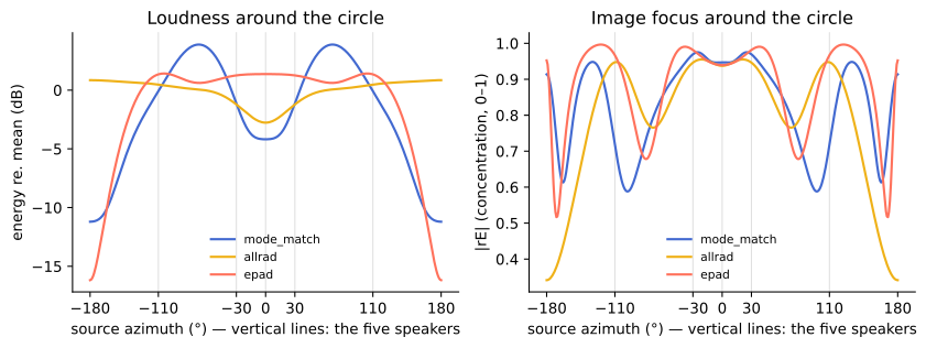
The figure is the guidance. On this gappy layout, mode_match and
epad swing 15–18 dB in loudness around the circle (listen to the left
panel: a source panned through the rear gap ducks, then blooms at the
surrounds); allrad holds loudness within ~4 dB everywhere. The right
panel shows the price: in the rear gap allrad's focus (|rE|) falls to
~0.4 — wide, wallpaper-soft imaging — where the others hold more focus
at the cost of that loudness rollercoaster. Nothing wins; the layouts
choose.
Choosing, as a table
| Your array | Reach for | Because |
|---|---|---|
| Regular ring or sphere (quad, hexagon, octagon, cube) at adequate order | mode_match (default) or epad | the inversion is healthy; you get maximum faithfulness, and the two nearly agree |
| Irregular / gappy (5.1, 7.1, 7.1.4, real venues) | allrad | even loudness beats sharp-but-lumpy on layouts with holes; this is what it was invented for (Zotter & Frank 2012) |
| Ring only, but the scene has height | epad or allrad | both handle the un-renderable height channels gracefully; naive inversion can misbehave |
| Undecided | A/B it — it's one message | decoder_type allrad etc.; rebuilds happen on a worker thread and crossfade in click-free, so switching mid-playback is a legitimate listening test |
And max_re 1, the attribute from Chapter 5, composes with all three:
it tapers the higher orders to concentrate energy (the psychoacoustic
optimum above the reconstruction limit — Chapter 7's sidebar). On real
speakers in real rooms it is almost always an improvement; the book's
default advice is simply on.
The room strikes back
The matrix assumes equidistant, level-matched, correctly-angled speakers. Chapter 5's tape-measure discipline covers the ideal case; real rooms add three adjustments worth knowing:
- Unequal distances (the sofa is against the wall): delay the near
speakers so wavefronts arrive together —
mc.delay~on the decoder's output cord, ~2.9 ms per meter of shortfall, before level matching. - Unequal speakers (the rears are smaller): match levels with pink
noise per speaker (Chapter 5), and accept that timbre will shift with
direction;
allrad's even energy makes mismatched speakers less conspicuous, one more point in its favor for found arrays. - A layout that isn't any preset: the preset list (Chapter 5's table) covers the standard rigs. For a genuinely custom array — the gallery's seven ceiling speakers — the library computes decoders for arbitrary speaker lists (it's one function call; the Max object currently exposes the presets), so a custom rig is a feature request or a small C++ patch away rather than impossible. Until then, pick the nearest preset and correct angles physically — moving a speaker beats lying to the matrix.
One loose end from Chapter 10: the nfc stage there compensates the
source's proximity. The speakers' own proximity (a desktop-radius
rig curves wavefronts too) is a further refinement — NFC-HOA per array
radius — that AmbiTap doesn't currently expose; at typical listening
radii (≥ 1.5 m) its absence is minor. Know the term, don't lose sleep.
The listening protocol
The companion patch wires the full A/B: an orbiting source, decode~ 3 surround_5_1 with the three decoder_type messages and the max_re
toggle, plus a binaural monitor branch for the speakerless. The
protocol that teaches fastest, on speakers or on the binaural stand-in:
- Orbit slowly with
mode_match. Hear the loudness swing as the source crosses the rear gap — the left panel of the figure, live. - Switch to
allradmid-orbit (it crossfades). Loudness levels out; listen for what softened in the rear. - Toggle
max_reboth ways on each. Cleaner concentration versus a hair of sparkle. - Park the source at −110° (a surround speaker) and A/B again — differences nearly vanish on a speaker; the philosophies only disagree between speakers.
Checkpoint
A decoder is one matrix and three philosophies: invert (mode_match),
re-pan (allrad), preserve energy (epad); gappy layouts favor
allrad, healthy ones favor inversion, max_re helps almost always,
and switching is a click-free message so your ears get the final vote.
Speakers handled — back to the other renderer, the one you carry in
your pocket. Binaural, properly, next.
Binaural, properly
ambitap.binaural~ has been quietly rendering your scenes since Chapter
3. This chapter opens that box: what an HRTF really is, why the object
offers two flavors of the same ears, when to bring your own, and how to
make headphone spatial audio survive contact with an audience of
strangers' heads.
Companion patch: patchers/booklet/08-binaural.maxpat.
The ears in the machine
Chapter 1's cues — timing, shadow, pinna spectra — can be measured: put microphones in the ear canals of a head, play a sweep from hundreds of directions, record what arrives. The result, direction by direction, is the head-related transfer function: a pair of filters that turn "a sound from over there" into "what each eardrum receives." Render a source by convolving it with the pair for its direction, and you've forged the complete cue set — which is all binaural rendering is.
AmbiTap's built-in head is KEMAR — the standard measurement mannequin (the MIT Media Lab's classic 1994 dataset), embedded in the library as a spherical-harmonic projection to order 5, resampled automatically to your session rate. Two consequences you've already experienced: it works with zero configuration, and its pinnae are not yours (Chapter 3's "elevation may feel vague").
Rendering a whole scene — sixteen channels of coincident patterns, not one source — works because the HRTF set itself can be expressed in the same spherical-harmonic language as the bus: the renderer convolves your scene channels with an SH-domain filter bank, and every source, room reflection, and recorded bird in the bus lands at both eardrums with the right cues, in one pass. That's why the object's cost is flat however crowded the scene gets (Chapter 9's scaling argument).
ls versus magls — the audible choice
The object's hrtf_dataset attribute offers two projections of the same
KEMAR measurements, and the difference is a genuine listening decision,
so here it is measured — the reconstructed ear responses at order 3 for a
hard-left source:
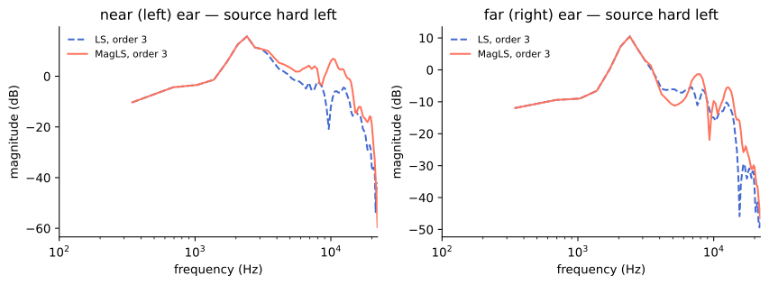
The issue: order 3 can't carry the full directional fineness of high-frequency ear acoustics (the same order-limit as everything else — Chapter 7). Above that limit, something must give:
ls(least-squares) keeps the waveforms as faithful as the order allows — phase, timing, everything — and pays by shedding high-frequency energy where the order runs out (the dashed line sagging at the shadowed ear above ~5 kHz). Sounds: duller, slightly in-the-head up top, with the most literal ITDs.magls(magnitude least-squares) declares high-frequency phase perceptually negotiable — above the limit your ears mostly read magnitude anyway — and spends the order budget holding the magnitude response instead (the solid line tracking full brightness). Sounds: brighter, more open, better externalization and high-frequency localization. The modern default recommendation, here and in the literature it comes from (Schörkhuber & Höldrich et al., 2018-vintage research; Appendix D).
A/B them in the companion patch (hrtf_dataset ls / hrtf_dataset magls — the swap crossfades) on cymbals or noise at a side angle. Most
listeners land on magls and stay.
Bringing your own ears: SOFA
Borrowed ears cap the ceiling (Chapter 7's rider #1). The industry's answer is the SOFA file (Spatially Oriented Format for Acoustics) — a standard container for measured HRTF sets, and the object accepts one:
[sofa /path/to/yours.sofa]      ← projected onto the SH basis at this
                                   object's order, resampled to the host
                                   rate; [sofa] with no path reverts to KEMAR
Where a personal file comes from, realistically, in 2026: an acoustics lab measurement (rare, wonderful), a photogrammetry service (apps that derive an HRTF from photos of your ears — commercial, variable, improving), or a chosen stranger — public databases (the HUTUBS and ARI collections, the SADIE II set, and others) hold dozens of measured heads, and picking the one that localizes best for you already beats the mannequin. Expect the biggest personal-HRTF gains exactly where the mannequin is weakest: elevation and front/back stability.
Head tracking, made real
Chapter 4 taught the principle (counter-rotate the scene) and the
division of labor (binaural~'s own yaw/pitch/roll are the
listener's head). What remains is plumbing: any device that emits
orientation — a phone strapped to headphones (free apps stream
gyroscope data as OSC), a dedicated tracker, a webcam face-tracker —
becomes three messages:
[udpreceive 7500] → [route /yaw /pitch /roll] → [yaw $1] etc. → [ambitap.binaural~ 3]
(Angles in radians as always; convert per your driver.) Rotation rebuilds happen off the audio thread and crossfade in, so tracker jitter doesn't zipper. Two rules of thumb from the VR world: total motion-to-sound latency under ~50 ms reads as solid; and even cheap tracking transforms realism, because Chapter 1's tie-breaker — cues that respond to your movement — matters more than cue perfection.
Craft notes for headphone delivery
- Externalization stack:
magls+ a room (Chapter 11 — one floor reflection outsells any HRTF upgrade) + head tracking if you have it. In that order of effort, that order of payoff. - Level: the renderer's
volumeattribute ramps smoothly — use it as the master, and mind that HRTF peaks can push hot mixes into clipping; leave a few dB. - EQ after, not before. Headphone-compensation or taste EQ belongs on the stereo output, downstream of the renderer; EQ on the bus changes the scene, EQ after changes the headphones.
- Strangers' heads: delivering binaural renders to the public means KEMAR-versus-everyone; expect front/back flips among listeners. Ship head-tracked (an app, a web player) when stakes are high; for a fixed file, favor material whose staging survives blur — motion, music, ambience over pinpoint statics.
Checkpoint
Binaural = measured ear filters; the bus renders through them in one SH
pass at any scene size; magls is the modern pick; SOFA opens the door
to better-than-mannequin ears; tracking is three OSC messages and pays
absurdly well. You can now render anything to anyone — next problem:
seeing what you're doing in a medium with no waveform display. The
scene needs instruments.
Watching the scene
Stereo engineers get meters, goniometers, spectrograms — a whole cockpit. Your medium so far has been sixteen channels of abstractly-aimed microphones, monitored through borrowed ears. When something is wrong ("why is the mix left-heavy? is it left-heavy?") you need instruments that answer about the scene, not about channel voltages. The package ships two, plus a set of gauges to put them on screen.
Companion patch: patchers/booklet/09-watching.maxpat.
The compass: ambitap.energyvec~
The scene's energy vector is the loudness-weighted average direction
of everything sounding — "where is the center of acoustic mass right
now?" ambitap.energyvec~ computes it continuously: the bus goes in,
three signals come out — x (front), y (left), z (up) — each in
−1…+1, smoothed over an adjustable smoothing_time.
One dominant source: the vector points at it (this is real direction-finding — the library verifies its DOA tracking against ground truth). A balanced full mix: the vector hovers near zero, and that is its quiet everyday use — a balance meter for the sphere. A mix that drifts left-heavy shows as y creeping positive long before you'd swear to it by ear. Because the outputs are signals, they're also patchable material: run y into a panner, a filter, a projector via OSC — the mix analyzing itself back into the art.
The map: ambitap.grid~
Where the compass gives one arrow, ambitap.grid~ gives the weather
map: it integrates the bus into a directional energy image — azimuth
across, elevation down, brightness = energy — the analysis behind this
figure (two noise sources, one 8 dB quieter; the white circles mark
their true positions):
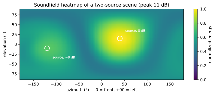
Note the honest blur: at order 3 each source paints a ~75°-wide blob (Chapter 7, now visible). You read this display for structure, not pinpoints: how many things, roughly where, how dominant, and whether energy lives where you think it does — the −8 dB source is plainly there, plainly secondary, plainly rear-right.
Mechanically the object is a passthrough plus a reporter: the bus flows
through unchanged; bang it (a qmetro 50 — display rate, not audio
rate) and it emits a grid <rows> <cols> <peak_db> <values…> list —
normalized energies ready for any display you like. Attributes:
azimuth_steps (resolution), smoothing_time (integration — long for
mix balance, short for watching movement), dynamic_range (how many dB
the brightness axis spans).
The cockpit
Lists and signals are instrument feeds; the package also ships the
gauges. Built with the externals (-DAMBITAP_MAX_BUILD_UI=ON, the
default when node is present) is a set of v8ui widgets — a
drag-to-aim panner, the heatmap (consuming exactly grid~'s
list), a DOA dot fed by energyvec~, per-speaker layout meters
for the decoder, and a rotation ball for rotate~ — with
patchers/ambitap.ui-tour.maxpat wiring all of them to a live scene at
once. The same widget set runs in a web browser as a remote control
surface over OSC (the library repo's ui/ layer). This book won't
re-document them — open the tour patch — but the companion patch embeds
the two essentials (heatmap + DOA) next to their raw-data views so you
can see the plumbing.
A monitoring practice
Instruments matter only inside a habit. A practice that fits on an index card:
- Park the compass on the master bus, always — smoothing ~1 s. Its job is the slow question: is the mix balanced on the sphere? Glance at it like you glance at a master meter.
- Raise the map when you're placing or hunting — smoothing short.
Two uses: confirm a placement went where you sent it (a
distance~typo that mutes a source is instantly visible as a missing blob), and find the actual direction of something misbehaving before reaching forvmic~(next chapter) to solo it. - Trust ears over instruments, in that order. The map shows energy, not perception: a 40°-wide blob can localize rock-solid (Chapter 7's max-rE psychoacoustics don't render on a heatmap), and the compass reads a hard-left source and a balanced chorus as the same near-zero when both coexist. Instruments answer "what is there"; only monitoring answers "how does it read."
- Meter the channels too, occasionally. Plain
mc.meter~on the bus still catches the prosaic disasters — a runaway encoder, DC, a channel-count mismatch — that scene-level instruments politely integrate away.
Checkpoint
Two instruments, two questions: energyvec~ — where is the center of
mass (balance, tracking, a patchable signal); grid~ — where is the
energy (structure, placement checks, a display feed); widgets in the
package put both on screen, and a four-line practice keeps them honest.
Now that you can see the scene, you can operate on it surgically — solo
a direction, duck a direction, flip the stage. Mixing inside the scene
is next.
Mixing inside the scene
A stereo engineer reaches into a mix constantly: solo this, duck that, flip the guitars, glue the bus. Chapter 2 warned that a scene-based format resists reaching in — the sources have already dissolved into the field. True, and yet the field itself can be operated on by direction, which turns out to cover most of what a mixer actually wants. Four objects, four moves.
Companion patch: patchers/booklet/10-mixing.maxpat.
Solo a direction: ambitap.vmic~
A virtual microphone: aim it into the scene (azimuth,
elevation) and it extracts a mono signal of what's sounding from
there — the max-rE beam from Chapter 3's figure, pointed by you
(max_re 1 for the clean pattern; off for the sharper, lobier one).
Uses, in ascending sneakiness: solo-in-place for the ear ("what is that at 140°?" — aim, listen, know); stems from a finished scene (aim four vmics at a recorded soundfield and you've derived a quad of spot mics that never existed); sidechain taps (the beam's output can key a compressor — duck the music when the narrator's direction speaks). Its resolution is the scene's order — at order 3 the beam is ~75° wide, a section mic, not a lavalier. It pairs naturally with the heatmap: find the blob on the map, aim the beam, listen.
Turn a direction up (or down): ambitap.directional~
The complement: instead of extracting a direction, reweight it, in
place, on the bus. azimuth/elevation aim it, gain sets what
happens there — below 1 to duck a region, above 1 to feature it — and
the rest of the sphere passes untouched (MC in, MC out; the transition
region is as wide as the order allows, so think broad tonal shaping of
the sphere, not surgical notches).
This is the scene's version of a mixer's most common move. The audience side of the room is too loud in the installation recording? Duck 30° of it 4 dB and leave the piece alone. The soloist needs 2 dB at stage-left? Feature the direction, not the stem you no longer have.
Flip the stage: ambitap.mirror~
Three toggles — flip_lr, flip_fb, flip_ud — each reflecting the
entire scene across a plane, instantly and losslessly (sign flips on
the appropriate channels; nothing is re-rendered, nothing blurs).
The workhorse is flip_lr: the mix-translation of a stereo
engineer's L/R swap. Check whether your staging survives mirroring
(balanced mixes mostly should); adapt a piece to a venue whose
geometry argues with your left-right choices; A/B suspicion about your
own ear's bias ("is the mix left-heavy or am I?" — flip it; if it
sounds right-heavy now, it was you). flip_fb earns its keep fixing
front/back-inverted recordings (a mic mounted backwards — it happens
more than anyone admits) and flip_ud fixes an inverted mic mount in
one click.
Glue without smear: ambitap.compress~
Compressing a scene channel-by-channel with sixteen ordinary compressors would be a disaster: each channel's gain would pump independently, and since direction lives in the gain ratios between channels (Chapter 6), independent pumping literally modulates where things are — sources lurch toward wherever the compression bites least.
ambitap.compress~ is built around the fix: it meters W only — the
omni channel, the scene's honest mono level — computes one gain
signal, and applies that same gain to every channel. Loudness breathes;
geometry is mathematically untouched (the channel ratios are preserved
exactly, which is why it's called image-preserving). The controls are
the familiar five — threshold, ratio, attack, release,
makeup_gain — behaving like every compressor you've ever set, just
aimed at a sphere. (Its static curve and attack/release clocks are
measured, not vibes — the library's behavior notebook plots them.)
Use it where you'd use bus compression in stereo: gluing a full scene,
taming a live input's swings before the encoder chain, limiting an
installation's output. What it deliberately cannot do is
multiband/multi-direction compression — squashing only the loud half
of the room — because that would be directional~'s aim with a
detector, and yes: vmic~ (detector) driving directional~ (gain) is
exactly how you'd patch that, all three objects consenting adults on
one bus.
The order of operations
A scene channel-strip, assembled from the four plus earlier chapters — a sensible master-bus order when you need everything at once:
sources & rooms → [mirror~] → [directional~ …] → [compress~] → [rotate~] → renderer
     (create)      (fix)         (reweight)         (glue)      (stage)
Corrections before creative reweighting; dynamics after the tonal
balance they should respond to; rotation last so everything upstream is
defined in scene coordinates, not performance coordinates. vmic~
hangs off the bus wherever you need an ear or a key signal — it's a
listener, not a link in the chain.
The companion patch builds a three-source scene and puts all four
objects on switches, with the Chapter 14 instruments watching. The
five-minute lesson: flip flip_lr while watching the heatmap (the map
mirrors, the compass's y negates — geometry moved, nothing else);
then drive the compressor hard and watch the map not move while the
level breathes.
Checkpoint
Reaching into a scene means operating by direction: extract one
(vmic~), reweight one (directional~), reflect them all (mirror~),
and control dynamics through one W-keyed gain so the image never
smears (compress~). Your mixes are now maintainable, not just
buildable. Two special-purpose renderers remain before the wider world
— first, the strange art of making two loudspeakers whisper binaural
signals into your ears.
Speakers pretending to be headphones
Chapter 13 ended with binaural rendering as your most portable renderer — with one string attached: headphones. The moment those signals play from two loudspeakers, physics vandalizes them: the left speaker reaches your right ear too (and vice versa), a few hundred microseconds late, filtered by your head. That's crosstalk, and it erases exactly the interaural differences the render worked to forge.
This chapter is about fighting back — crosstalk cancellation (XTC, also transaural audio): pre-processing the two speaker feeds so that, at one listener's ears, the crosstalk arrives pre-cancelled and the binaural illusion survives open air. It's the most conditional trick in the book, which is why it gets the book's most honest chapter.
Companion patch: patchers/booklet/11-transaural.maxpat.
The idea in one paragraph
The path from two speakers to two ears is four filters (each speaker to each ear — measurable head acoustics, the same KEMAR data as Chapter 13). Those four filters form a 2×2 system; invert it, and you get four correction filters that make the acoustic journey undo itself: feed the corrected signals to the speakers and what lands at your ears is (approximately) the original binaural pair. Each speaker emits a precisely timed, filtered anti-copy of the other's crosstalk; the air does the subtraction at your head.
The catch is the word your: the inversion assumes a specific head at a specific spot. Move, and the cancellation unravels.
The object
binaural stereo (e.g. [ambitap.binaural~ 3] or a binaural file)
    |         |
[ambitap.xtc~]           ← geometry: span, distance
    |         |
two LOUDSPEAKERS         (never headphones — the "correction" would
                          itself be the artifact)
You tell it the geometry it must invert: span (the full angle
between the speakers as seen from the listening position, degrees) and
distance (listener to speakers, meters). Change either and the
filters are redesigned from the KEMAR model — off the audio thread,
crossfaded in, like every rebuild in the package. regularization
(0–1) trades cancellation depth against filter aggressiveness — lower
digs deeper but rings harder and breaks more brittly off-center; the
default 0.5 is a sane perch.
Two built-in honesties to plan around: the object adds 512 samples of
latency (~11 ms at 48 kHz), and its output sits about 12 dB below
bypass — headroom the aggressive inverse filters require. That's what
the ramped bypass attribute is for: it level-compensates comparison
poorly if you just flick it, so the companion patch A/Bs through a
+12 dB trim on the processed path, per the library's own listening
protocol. (The filter design itself is gated by measured tests in the
library — in-band cancellation depth among them — so what you're
tuning is geometry and taste, not whether the math works.)
What it's actually for
Where XTC earns its keep — the honest list:
- The desktop. One person, a meter from a stereo pair, head naturally steady: the near-ideal case. Personal near-field spatial audio without headphone fatigue. (Narrow spans work; the designer accepts 5–120°, and research systems favor very narrow "stereo dipole" spans for exactly this seat.)
- The demo chair / sweet-spot installation. A gallery piece with one seat; a listening-bar setup; the client preview chair. Staged deliberately — a marked seat is part of the piece — it's magical.
- Curiosity and craft. Hearing a fly circle your head from two visible speakers rewires your respect for interaural cues faster than any diagram.
And the disqualifying conditions, equally honest: more than one simultaneous listener (the correction for seat A is garbage at seat B), audiences that move, reverberant rooms (the room's reflections re-introduce uncorrected paths — dry rooms and near-field setups survive best), and anything where 11 ms of extra latency hurts. For those, decode to speakers (Chapter 12) like a sensible person; XTC is a scalpel, not a PA.
Note also what the signal path implies: XTC renders binaural
material. Your ambisonic scene reaches it through binaural~ — so the
full chain is scene → binaural render → crosstalk-cancel → two
speakers, and everything you know about the binaural stage (MagLS,
SOFA ears, head-tracking-less front/back flips) still applies at this
one's input.
The experiment
The companion patch: an orbiting scene through binaural~ into
xtc~, the trim-matched A/B, and geometry controls. Sit accurately
(tape measure; enter the true span and distance — self-reporting
flatters), then:
- Orbit with
bypass 1(plain stereo playback of a binaural render): the image lives between the speakers, Chapter 1's narrow window. - Engage. The orbit should leave the speakers — sides opening beyond the span, rear content plausibly behind. Depth of the effect varies with your head-vs-KEMAR similarity and the room's dryness.
- Now lean half a meter left. Watch the sphere collapse back into two speakers. That collapse is the chapter: you've heard both the power and the contract.
patchers/ambitap.xtcdesigner.maxpatshows the filters themselves redesigning as you drag the geometry — worth two minutes to see what you're listening through.
Checkpoint
XTC inverts the speaker-to-ear acoustics for one head at one spot: binaural in, two speakers out, geometry told truthfully, regularization to taste, 512 samples and −12 dB as the cost of doing business — a one-listener scalpel that's the wrong tool for every audience larger than one. Last craft chapter next, and it points the other direction entirely: not rendering scenes out, but folding the channel-based world in.
Beds and stems
The last craft chapter faces the direction we've ignored since Chapter 2: backwards, toward the channel-based world. Your collaborators live there. Sessions arrive as 5.1 stems; sample libraries ship quad ambiences; the sound designer's handoff is a 7.1.4 print. None of it is ambisonic, all of it is useful, and one object annexes it.
Companion patch: patchers/booklet/12-beds.maxpat.
The move
A channel-based bed is speaker feeds for a known layout — which means every channel has a defined direction (L = +30°, RS = −110°, …). So encode each channel at its canonical direction and sum:
[your 5-channel stem]              (one mc cord, L R C LS RS order)
    |
[ambitap.bed2hoa~ 3 surround_5_1]
    |
   bus — an ordinary ambisonic scene now
ambitap.bed2hoa~ takes the same <order> <layout> arguments and the
same layout list as decode~ — it is, conceptually, that object's
mirror image (decode: scene → feeds; bed2hoa: feeds → scene). The
matrix is static (directions don't move), so it's among the cheapest
objects in the package. Once through it, the material is scene:
rotatable, mirrorable, re-decodable to any rig, binauralizable —
the whole of Part III applies.
What the move is worth
Concretely, with the 5.1 stem session that just landed:
- Monitor it on headphones, properly.
bed2hoa~ 3 surround_5_1→binaural~ 3is an instant, correct virtual 5.1 room — each stem channel rendered from its true angle. For anyone who's mixed surround on a laptop, this alone justifies the object. - Re-deliver it anywhere. The 5.1 print, through the scene, decodes
to your quad rig, an octagon, or a dome (Chapter 12 rules apply —
allradfor the gappy targets). This is up/down/cross-mixing done by geometry instead of by folklore fold-down coefficients. - Use it as a bed in the Atmos sense: channel-based ambience layer underneath object-like foreground — here, encoded foreground sources (Chapter 9) summed onto the same bus as the imported bed. One cord, both paradigms, everything rotates together.
- Rescue legacy work. Quad tape-music realizations, 5.1-era installations — re-staged into scenes, they stop being hostage to one speaker count.
And the disclaimer, since this object is where wishful thinking
congregates: this is not upmixing magic. A bed encodes as five (or
eleven) virtual speakers on the sphere — phantom images between them
stay phantom (a source panned L↔C in the original is two correlated
virtual speakers, not a true 15° source), and the scene inherits the
bed's spatial resolution forever. bed2hoa~ relocates a channel-based
mix faithfully; it cannot un-bake the panning decisions inside it.
The LFE, finally
Every layout in this package has been "no LFE" since Chapter 5, with promises. Here's the whole policy in one place.
The LFE channel (the ".1") is a delivery convention — a separate low-frequency effects track for a subwoofer — not a direction. An ambisonic scene describes directional sound, and sub-bass direction is barely perceptible (which is why one subwoofer suffices in the first place). So the bus simply does not carry it, and the routing is:
- Importing a 5.1-with-LFE stem: peel channel 4 (the LFE) off
before
bed2hoa~—mc.unpack~, feed the five mains to the object, and route the LFE directly to your subwoofer output (or, on a sub-less monitor rig, mix it into the render at −∞ to −10 dB per taste; it's effects seasoning by definition). - Delivering to an LFE-expecting format: decode the scene to the mains (Chapter 12), and derive the LFE as a low-passed mono sum (W, low-passed, is the classical choice) — or better, keep true LFE-type material (the explosion sweetener) on its own mono track through the whole project, outside the bus, and print it directly.
- Bass management (rerouting mains' low end to the sub) is the monitor controller's job or a crossover after the decoder — playback plumbing, not scene content. Keep it downstream and out of the master.
The companion patch builds a synthetic 5.1 bed (five distinct sources
mc.combined in canonical order — front trio, rear pair), folds it in,
and renders binaurally, with the Chapter 14 heatmap showing five tidy
blobs at the canonical angles: the bed, visibly staged on the sphere.
Rotate it — five blobs turn as one — and the point of the whole
exercise lands.
Checkpoint — and the end of the craft
Beds fold in by encoding each channel at its canonical angle
(bed2hoa~, decode~'s mirror); the result is honest scene material
with the bed's resolution baked in; the LFE routes around the bus in
both directions.
Take stock: sources, distance, rooms, decoding, binaural, instruments, scene-mixing, XTC, beds. That is the complete AmbiTap toolkit and — by this book's argument — a complete spatial audio education in one package. Part IV takes exactly this skill set and shows you the same ideas wearing other uniforms: Pd, microphones, DAWs, game engines, and the A-word.
The same patch in Pd
Everything you've learned rides a bus, not a brand. This chapter proves it the quick way: Chapter 3's first-sounds patch, rebuilt in Pure Data, plus the complete phrasebook for moving any patch in this book between the two environments.
If you don't use Pd, skim the phrasebook table and move on — the real
lesson is how little changes. If you do: the companion patch is
booklet/01-first-sounds.pd in the AmbiTap-Pd repository.
Setup
AmbiTap-Pd ships the same DSP as the Max package — the identical
library underneath, wrapped as one Pd library named ambitap
containing all the ambitap.*~ classes. Requirements: Pd ≥ 0.54
(the first release with multichannel signal cords — the whole
architecture depends on them) and a build of the library
(cmake -B build && cmake --build build in the repo; the result lands
in externals/). Then, in any patch that uses the objects:
[declare -lib ambitap]
— the one line of ceremony Max's package system did for you.
First sounds, translated
[noise~]
|
[ambitap.encode~ 3]        ← same name, same creation arg, same
|                             (order+1)^2-channel multichannel cord
[ambitap.binaural~ 3]
|         \
[dac~]
Structurally identical. The differences are all dialect:
- Messages instead of attributes. Pd has no attribute system, so
parameters arrive as messages on the left inlet — same names, same
units:
[azimuth $1(,[elevation $1(,[yaw $1(. Radians here too; the[expr $f1 * 3.14159265 / 180]idiom survives unchanged. - Thick cords, same meaning. Pd ≥ 0.54 draws multichannel
connections like any signal cord;
[snake~]/channel tools apply if you need to split. Summing buses by joining cords works exactly as in Max. - No
@attr argsin the object box. Creation args carry the order/layout ([ambitap.decode~ 3 quad]— identical); everything else is a message after creation (a[loadbang]-driven message box replaces Max's saved attribute values).
The phrasebook
| Concept | Max | Pd |
|---|---|---|
| Load the objects | package in Packages/ | [declare -lib ambitap] |
| Set a parameter | azimuth 1.57 message or @azimuth attribute | [azimuth 1.57( message |
| Initialize a parameter | saved attribute | [loadbang] → message |
| The HOA bus | thick mc. cord | thick multichannel cord (Pd ≥ 0.54) |
| Watch the bus | mc.scope~ / mc.meter~ | per-channel via channel-splitting + [env~]s (no mc scope built in) |
| Multichannel output | mc.dac~ 1 2 3 4 | [dac~ 1 2 3 4] fed via channel-split |
| Audio on | ezdac~ / Audio On | DSP toggle (Media → DSP On) |
Object-for-object, the Pd library carries sixteen of the seventeen
Max externals — everything except ambitap.grid~ (the heatmap
analysis feed; its consumer is the Max v8ui widget layer, which has
no Pd counterpart yet). The whole of Parts I–III therefore translates,
with three practical footnotes from the Pd wrappers' own docs: the
convolution-based objects (binaural~'s SOFA loading is Max-only —
Pd's binaural~ uses the built-in KEMAR set with ls/magls intact;
panbin~, xtc~, room~) (re)allocate when the DSP graph compiles
and want power-of-two block sizes; xtc~ takes its stereo program on
two ordinary signal inlets; and the UI story is patch-it-yourself —
Chapter 14's instruments exist (energyvec~ outputs its x/y/z
signals identically) but the gauges don't.
Why bother?
Because the two environments have different superpowers, and scenes travel between them losslessly (it's the same AmbiX bus; record it to a multichannel file in one, open it in the other):
- Pd is deployable. It runs headless on a Raspberry Pi bolted inside an installation plinth, boots from a script, and costs nothing to license on ten machines. The economical pattern: compose in Max with the widgets and comforts, exhibit in Pd — same objects, same rendering, order-3 binaural comfortably within a Pi's budget.
- Pd is embeddable. libpd puts a Pd patch inside an app or game prototype; your spatializer rides along.
- And the reverse: if you live in Pd and borrowed this book for the concepts — everything in Parts 0–III holds verbatim; only the screenshots were in the other church.
Checkpoint
Same library, same bus, same names, same radians; messages for
attributes, declare -lib for the package, sixteen of seventeen
objects, no widget layer. Skills, it turns out, were never
Max-shaped. The next three chapters push that further — into
microphones, DAWs, and game engines — where even the object names stop
being familiar but the ideas keep translating.
Recording a scene
Everything so far synthesized scenes. But Chapter 2 flagged the scene-based paradigm's exclusive: it's the one you can point a microphone at. A single instrument on a stand captures the actual soundfield of a forest, a cathedral, a protest, a rehearsal — behind, above, all of it — as a bus your whole toolkit already speaks.
This chapter is the field guide's field chapter: how the microphones work, what the market looks like, and the craft that makes location B-format worth keeping. (Ecosystem facts here are stated as of 2026; models drift, principles don't.)
A-format and B-format
Chapter 6's ideal — an omni and three figure-8s occupying one point — cannot be built; microphones have bodies. The 1970s solution (Gerzon and Craven's, still the standard design) is the next best thing: four cardioid capsules on the faces of a tiny tetrahedron, as close to coincident as manufacturing allows.
The raw four-capsule output is called A-format — four aimed
cardioids, useless directly. But within the coincidence approximation,
sums and differences of the four reconstruct the ideal set exactly:
all four capsules summed ≈ the omni W; front pair minus back pair ≈
the X figure-8; and likewise Y and Z. That matrixing (plus filters
correcting the "tiny but not zero" spacing) is the A-to-B
conversion, and it ships with every mic as a plugin or is done
on-board. The output is B-format — and after Part II you know
precisely what that means, down to asking the professional's three
questions (order? channel order? normalization?). Modern mics emit
AmbiX; vintage material and the classic SoundField lineage speak FuMa;
format~ (Chapter 8) stands at the border.
Higher orders need more capsules — the (N+1)² economics again, now in hardware: order 2 wants ~8+ capsules, order 4 wants ~32 arranged on a rigid sphere, and the conversion mathematics gets correspondingly heavier. This is Chapter 7's "microphones lag encoders," explained.
The market, in tiers (2026)
- Recorder-integrated, first order. The Zoom H3-VR class: four capsules, A-to-B conversion, level-metering and an SD card in one handheld box. The field-recording workhorse tier — point at the world, get AmbiX WAV.
- Studio-grade first order. The Sennheiser AMBEO VR, Rode NT-SF1, and the SoundField heritage line (now under RØDE/Freedman): better capsules, XLR outputs, conversion in a plugin where you can choose the output convention. The tier for material that will be mixed hard.
- Higher-order arrays. Spherical rigid arrays: Zylia's ZM-1 class (order ~3 from 19 capsules) and the research-and-broadcast Eigenmike em32/em64 (orders 4–6). Costs jump an order of magnitude; so does the post-processing. Rent before buying; verify your whole chain handles the channel counts.
- Adjacent but not ambisonic: binaural head rigs record two-channel
ear signals (lovely, but baked — Chapter 13's format, not a scene),
and spaced multichannel trees capture enveloping channel-based
material (fold it in with
bed2hoa~if you must, remembering what it is).
Field craft
The handful of practices that separate keeper B-format from expensive regret:
- Orientation is sacred. The mic's marked front is your scene's
0° forever after. Photograph the setup; note "front = stage" in
the slate. A mounted-sideways surprise costs an afternoon of
rotate~forensics (and an upside-down one is whyflip_udexists — Chapter 15's rescue list, written from experience). - The mic is the listener's head. Where you stand it is where every future listener stands. Height matters (ear height reads natural; 3 m up reads crane shot). Proximity matters doubly: nearby sources dominate a coincident array fast — the "step back" your recording teacher preached, now in 360°.
- Wind and handling travel in W. Standard protections (blimps, suspensions) apply — fourfold. Any thump is omnipresent by definition.
- Monitor binaurally on location: mic →
binaural~ 1is a two-object patch (or the recorder's own binaural fold-down), and it catches the orientation and proximity mistakes while they're still fixable. - Slate the paperwork: order, convention (the recorder's manual knows), sample rate, and orientation notes, in a text file beside the WAVs. Chapter 8 predicted this file; be the collaborator who ships it.
Recorded scenes in the toolkit
Back home, a recorded scene is just a bus with weather in it — every Part III tool applies. The idioms that come up constantly:
- Re-aim in post:
rotate~turns the whole location; the take where the action drifted 40° left is salvageable. - Interview the field:
vmic~beams extract usable mono spot "mics" from a scene recorded with none (order-limited, but astonishing the first time). - Recorded bed + synthetic foreground — the hybrid Chapter 7 recommended: first-order forest as the world, order-3 encoded sources as the story. Sum the buses (pad the first-order scene's 4 channels into the order-3 cord) and the seam is inaudible.
- Stabilize handheld moves the same way VR does: record the mic's orientation (IMU or careful notes), counter-rotate in post — Chapter 4's head-tracking machinery, pointed backwards in time.
Checkpoint
Tetrahedra of cardioids → A-format → matrixed to B-format; first order is a handheld commodity, order 4+ is a spherical-array specialty; orientation, placement, and paperwork are the craft; and a recording is just a bus you didn't have to patch. One question remains before the DAW chapter poses it everywhere: your scenes — synthetic or recorded — eventually have to ship. Onward to the toolchains the rest of the industry mixes in.
The DAW route
Not every spatial project wants a patcher. Long-form editing, comping, automation lanes, video sync, stem management — the things DAWs are for — don't stop mattering because the mix has a Z axis. This chapter maps the DAW route to the same destination: which host, which plugin suites, and how the concepts you own translate. (Names and versions as of 2026; the shape of the route changes slowly.)
The host question
An ambisonic mix needs tracks and buses that carry (N+1)² channels through plugin chains without flinching. That single requirement sorts the DAW market:
- Reaper is the community's default answer, and this chapter's: tracks up to 128 channels, per-track channel mapping, plugin pin routing, multichannel files as first-class citizens — order 7 rides an ordinary track. Cheap, scriptable, cross-platform.
- Pro Tools, Nuendo, Logic carry ambisonic bus formats natively but historically cap them low (commonly order 3, tied to their Atmos-centric workflows); fine for delivery work inside those ecosystems.
- Ableton Live and the performance DAWs have no native ambisonic bus; the working pattern is Max for Live devices (your Part I–III patches, literally, hosted in a set — see Envelop below) with multichannel routing tricks.
The rest of this chapter assumes Reaper; translate freely.
The plugin suites
Four open-source suites cover the territory; all speak AmbiX; a working mix borrows from several (they chain happily — it's all the same bus):
- IEM Plug-in Suite (Graz — the institute whose research this
book keeps citing): the reference set. Encoders, a SceneRotator,
AllRAD-based decoding with a decoder-designer, binaural, EnergyVisualizer
— plus the celebrated RoomEncoder (a positional room simulator
in the spirit of
room~, with hundreds of image-source reflections). Order 7. If this book had a DAW edition, it would be written over IEM. - SPARTA (Aalto): the research bench — up to order 10, SOFA
binaural with OSC head-tracking, spherical-array encoders (your
Eigenmike's A-to-B stage lives here as
array2sh), beamformers, powermaps (Chapter 14's instruments, DAW edition), and the parametric COMPASS processors. - ambiX plugins (Kronlachner): small, ancient, indispensable —
converters (the
format~of the DAW world), rotators, and the ambiX binaural/decoder pair that half the field's tutorials assume. - ATK (Ambisonic Toolkit) for Reaper: first-order-focused
classics with a strong transform vocabulary (dominance, focus —
directional~'s relatives) and deep documentation lineage. - Envelop for Live: the Ableton answer — Max for Live devices (order 3) for source panning, rotation, and binaural monitoring, born from the Envelop venue's practice.
Concept-mapping is one row each: encode~ → any suite's encoder
("panner"); rotate~ → SceneRotator; decode~ → the suite decoders
(IEM's designer covers the custom-array case Chapter 12 wished for);
binaural~ → the binaural decoders; grid~/energyvec~ → the
visualizers. Your Part III instincts — order choices, ALLRAD-for-gappy,
MagLS, W-keyed dynamics — transfer without edits.
The session template
The load-bearing trick: the master bus is an ambisonic bus. In
Reaper: set the master (or a dedicated "SCENE" bus track) to 16
channels for order 3; every source track gets an encoder plugin as
its panner and sends multichannel to the scene; the scene's chain
ends in a monitoring section — a binaural decoder for headphone
work, a speaker decoder when the rig is attached — that you bypass
at render time when delivering the raw scene. AmbiTap fits this
picture at the borders: record your Max scene to a 16-channel file
(mc. recording into sfrecord~-style workflows) and it drops onto
the Reaper timeline as a finished element; conversely a Reaper-mixed
AmbiX render walks into any patch in this book.
Automation is where the DAW route earns its keep — encoder azimuths drawn against picture, order-3 beds under comped dialogue — and the one habitual mistake is putting channel-ignorant plugins on the scene bus: a stereo compressor inserted on 16 channels processes two and passes fourteen, smearing geometry Chapter 15 taught you to protect. Scene buses take scene-aware processors only (IEM ships multiband dynamics; the W-keyed trick is portable); source tracks, pre-encoder, take anything.
Delivery
The last mile, format by format:
- Scene masters: multichannel WAV, AmbiX, order stated — the Chapter 8 paperwork. This is the archival master everything else renders from.
- YouTube 360 / VR video: first-order AmbiX (4ch) muxed with the video, plus optionally a head-locked stereo track; Google's injection tooling stamps the metadata. Truncate your order-3 master (Chapter 7's nesting — drop channels 4–15), check the result binaurally, done.
- Binaural print: render through your best binaural decoder (MagLS, personalized ears if you have them) to plain stereo. State "binaural — headphones" on the file; it's a render, not a scene (Chapter 13's caveats about strangers' heads apply).
- Speaker prints: decode per venue (Chapter 12), print the feeds, label the layout. For festival-circuit work, ship the scene plus a README instead and let each venue decode — the entire point of the format.
- Atmos deliverables: a different paradigm, not a different button — the next-but-one chapter untangles it.
Checkpoint
Reaper (or any wide-bus host) + IEM/SPARTA/ambiX/ATK covers the DAW route end to end; the session pattern is encoder-as-panner into a scene-format master bus with monitoring you bypass at render; delivery is AmbiX for scenes, truncation for YouTube, renders for binaural and rigs. Same bus, longer timeline. Next: the toolchains where the listener steers — games and XR.
Games and XR
Interactive audio is where every thread of this book was already braided together decades ago — object rendering, scene beds, binaural output, head tracking — because games never had a choice: the listener steers. This chapter maps that world's architecture onto your vocabulary, so when you walk into a game-audio pipeline (or ship a VR piece) you recognize everything. Names as of 2026.
The standing architecture
Every serious engine pipeline converges on the same three-layer design — which Chapter 9 already taught you in miniature:
- Foreground: objects. Each emitting thing (footstep, voice,
engine) is a mono source + position, rendered per frame relative
to the listener — the object paradigm, panned to speakers or
convolved per-source to binaural (
panbin~was this, one object at a time). Sharp, interactive, per-source cost. - Background: an ambisonic bed. The forest, the city, the room tone — authored or recorded as B-format (Chapters 3–19!), carried as one bus, and counter-rotated with the listener's head each frame. One matrix multiply for the whole world's ambience — Chapter 4's economics, deployed at industrial scale. This is the reason VR standardized on Ambisonics.
- Output: binaural (or the room's speakers). On headsets, both layers render through HRTFs; head tracking comes free from the HMD at far better than Chapter 13's 50 ms budget.
Middleware names for the same picture: Wwise ships ambisonic busses (to 5th order) alongside its object pipeline; FMOD routes ambisonic assets through spatializer plugins; engine-native audio in Unity/Unreal accepts first-order AmbiX ambience assets and delegates rendering to a pluggable spatializer. The spatializer SDKs you'll meet by name: Steam Audio (Valve — notable for tracing actual geometry to drive occlusion and reflections), Meta XR Audio (the Quest lineage), and Resonance Audio (Google's open-source engine — ambisonics-based internally, order 3, now dormant but instructive and still deployed). Under every one of those logos: encode, rotate, decode binaurally — your Part I patch, shipped at 90 fps.
What translates, and what's new
Carrying your skill set in:
- Order economics (Chapter 7) reappear as performance budgets: engine beds run orders 1–3 because the rotation and decode happen per frame on consumer hardware, next to the game. Your instinct for "what does order 1 blur sound like" is directly a shipping decision.
- The bed/foreground split (Chapter 9's fork) is now enforced by architecture: precious sources go objectward, diffuse world goes busward. You've already practiced the judgment.
- Rooms (Chapter 11) become acoustics systems: image-source
thinking survives, but engines trace real level geometry (Steam
Audio bakes or ray-traces reflection paths).
room~'s mental model — direct/early/tail, geometry drives the earlies — is exactly the right preparation. - Authoring is where AmbiTap re-enters: engines consume first-order (sometimes order-2/3) AmbiX WAV as ambience assets. Your Max rig — encode, room, mix, record the bus, truncate per Chapter 7 — is an ambience-asset production line. (And a Pd patch via libpd, Chapter 18, is a legitimate prototyping spatializer.)
Genuinely new, worth respecting: occlusion and propagation (walls muffle, sound bends through doorways — driven by game geometry, no Part III equivalent), interactive mixing (snapshots and side-chains driven by gameplay state), and voice budgets (the renderer is sharing a CPU with a game; everything is priority-managed). Game audio is its own deep craft — this chapter's claim is only that its spatial layer is your Part I–III knowledge wearing a hard hat.
Shipping a small VR piece — the shape of it
For the common near-term case — a 360 video or a modest headset experience — the pipeline in five lines:
- Compose the world as an order-3 scene in Max (everything you know).
- Print: full scene for archive; order-1 truncation for the video platforms (Chapter 20's delivery table).
- For real-time pieces: import the bed as AmbiX into Unity/Unreal + a spatializer SDK; author foreground as objects.
- Let the HMD drive rotation (never hand-roll what the runtime provides).
- Test on the actual headset early — Chapter 13's strangers'-heads caveats apply to every player, and loudness targets differ from music norms.
Checkpoint
Games render foreground as objects and world as head-tracked ambisonic beds through binaural output; the middleware names change, the architecture doesn't, and your order/bed/room instincts are the transferable core. One name has been conspicuously deferred through this whole part — the one on every client brief. Atmos, next.
Atmos and friends
Somebody is going to say it in a meeting: "can we get this in Atmos?" This chapter equips you to answer — what Dolby Atmos actually is, how it relates to the scenes you now build fluently, when each paradigm genuinely wins, and the workflows where they cooperate. Tone check before we start: this book is not against Atmos. It is against fog. (Specifics as of 2026.)
What Atmos actually is
Dolby Atmos is the object-based paradigm from Chapter 2, shipped at industrial scale with a licensing program attached:
- A mix is beds + objects: channel-based base layers (typically 7.1.2-shaped) plus up to ~118 mono/stereo objects, each with positional metadata authored against a standardized renderer.
- The renderer is Dolby's. At playback — cinema processor, AVR, soundbar, phone — Dolby's renderer lays objects onto whatever speakers exist, or into its binaural mode for headphones. Authoring happens through the Dolby Atmos Renderer application (or DAW-integrated equivalents in Pro Tools/Nuendo/Logic; Apple's ecosystem wraps the same delivery as "Spatial Audio").
- The deliverable is a master file (ADM BWF / IAB families), and distribution runs through platforms licensed to decode it.
Read that against Chapter 2's table and the trade is familiar: maximum per-object discreteness and a consumer-delivery pipeline that works at retail scale, in exchange for spatial decisions finalized by a renderer you don't control, on speaker layouts you'll never see.
Scene versus object, without the marketing
Where each paradigm genuinely wins — the honest scorecard your meeting needs:
Atmos wins consumer delivery (the only spatial format with end-to-end reach into living rooms, cars, and earbuds), discrete foreground precision on dense speaker rigs, industry interop (dubbing stages, streaming specs, loudness pipelines), and any brief where the deliverable is "an Atmos master" — by definition.
Ambisonics wins rotatability (nothing head-tracks a finished Atmos mix outside Dolby's own binaural path; a scene rotates for one matrix — Chapters 4, 21), recordability (there is no Atmos microphone; there are ambisonic ones — Chapter 19), diffuse material (Atmos objects are points; a scene is a field), venue independence outside the licensed ecosystem (your dome, your gallery, your festival decode — Chapter 12), archival transparency (a math-defined open bus versus a renderer-defined proprietary master), and cost (zero licensing, this entire toolkit).
Neither list embarrasses the other. They're different answers to Chapter 2's question, optimized for different economies.
Cooperation workflows
The practical part: the two paradigms meet constantly, and the crossings are well-trodden.
Scene → Atmos (the common direction: you composed spatially, the label wants Atmos):
- Decode into the bed: render your scene to 7.1.4 (Chapter 12 —
allrad, since that's a gappy layout) and deliver it as the Atmos bed. The scene's spatial character survives at the bed's resolution. This is the standard route for ambience/texture-heavy material. - Re-author the foreground as objects: your handful of featured sources — whose positions you have as automation already — become Atmos objects with the same trajectories, riding above the decoded bed. Bed-for-world, objects-for-story: the game-audio split (Chapter 21), performed one final time at delivery.
- What doesn't exist: a lossless "HOA in, Atmos out" button. The paradigm translation is real work; budget it.
Atmos-adjacent material → scene: a 7.1.4 print folds into your
bus via bed2hoa~ (Chapter 17, built for this) for monitoring,
re-staging, or archival — with that chapter's honesty about baked
panning. Object stems (dry source + position notes) port even
better: re-encode them as Chapter 9 sources and the piece is native
scene again.
Both-masters projects: keep the mix in stems + position data as long as possible (source-and-trajectory is the truly portable representation — more portable than either delivery format); print the scene master and the Atmos master as two renders of the same decisions. Studios doing regular spatial work converge on exactly this.
The other friends
Same paradigm-mapping, quickly: MPEG-H — the broadcast-world object/scene hybrid (notably: it can carry HOA natively — the one mainstream delivery family where your scene ships as itself; adoption is strongest in broadcast and parts of streaming). AURO 3D — channel-based height, a tall Chapter 2 column A. IAMF (AOM's open "Eclipsa" format, backed by Google/Samsung) — a young, royalty-free object/scene container to watch; ambisonic payloads are in its spec. If any of these is on your brief, the Chapter 2 table plus this chapter's scorecard method answers it.
Checkpoint
Atmos = beds + objects + Dolby's renderer + licensed delivery: the
object paradigm productized. It beats scenes at retail reach and
discrete precision; scenes beat it at rotation, recording, diffusion,
open venues, and price. They cooperate via decode-to-bed,
objects-for-foreground, and bed2hoa~ back — and "can we get this
in Atmos?" now has a costed, honest answer.
That completes the wider world. Every paradigm, toolchain, and delivery route is now on your map — which means it's time for the chapter this book was named for: given a situation, which tool?
The decision guide
Everything in this book converges here. You have a project; the field has a dozen tools; the promise of a field guide is that these two facts meet in minutes, not weeks. This chapter delivers the promise twice: first as questions, then as worked scenarios.
The four questions
Nearly every spatial audio decision resolves from four axes:
1. What's the deliverable — a scene, feeds, or a platform master? If the venue varies or the listener steers: scene (Ambisonics). If one known rig defines the piece: channel feeds. If a commercial platform names the spec: that platform's paradigm, full stop (Chapter 22).
2. Who's listening, on what? One tracked head (VR/binaural), many untracked heads on headphones (Chapter 13's caveats), one sweet seat (XTC territory), or a room of wanderers (arrays; order and decoder choices per Chapters 7 and 12)?
3. Is the material discrete, diffuse, or both? A few precise
foreground sources lean object-wise (panbin~, engine objects, Atmos
objects). Fields, rooms, and weather lean scene-wise. "Both" is the
professional's default answer, and the bed + foreground split (Chapters
9, 21, 22) is the standing solution.
4. What are the budgets? Channel count and CPU (order economics,
Chapter 7), latency (room~'s 53 ms, xtc~'s 512 samples),
licensing (open bus vs. platform), and the scarcest one — setup time in
the venue (Chapter 5's monitor-binaurally-decode-on-site discipline).
Answer four questions, and the scenarios below mostly write themselves.
Worked scenarios
Live electronics set (club/venue, rig varies per gig).
Compose order-3 in Max; master bus per Chapter 15; monitor binaurally
in rehearsal. Per venue: decode~ to the house layout — allrad,
max_re 1 for whatever gappy array exists (Ch. 12) — with Chapter 5's
tape-measure hour. Keep a stereo decode on a fader as the soundcheck
insurance policy. Why not objects/Atmos: no renderer at the club;
the scene decodes anywhere.
Gallery installation, speaker dome, three months unattended. Author in Max with the widgets; exhibit per Chapter 18: Pd headless on a small computer, same objects, decoded to the dome; order 3–4 if the dome is dense (Ch. 7's wandering-audience case for higher order). LFE/subs via W-derived send (Ch. 17). The trap to avoid: composing on the dome. Compose binaurally, calibrate on site.
VR title / 360 video. Foreground as engine objects; world as ambisonic beds authored on your Max production line and delivered as AmbiX WAV (order 1–3 per platform); HMD rotation does the head tracking (Ch. 21). For plain 360 video: order-1 AmbiX + head-locked stereo, injected metadata (Ch. 20). Why not pure scene: foreground sharpness; why not pure objects: the world would cost per-raindrop.
Binaural fiction / podcast drama (headphones, no tracking).
Order-3 scene; magls; room per scene from Chapter 11 (the
externalization stack); featured close voices via panbin~ (Ch. 9's
fork); print per Chapter 20. Favor motion and staging that survive
front/back ambiguity (Ch. 13). Why not Atmos: Dolby's binaural is a
platform render; here you are the renderer and can voice it.
Commercial music release "in Atmos."
The spec answers question 1: author beds + objects against Dolby's
renderer (Ch. 22). Your kit still earns its keep upstream — spatial
sketching, ambience design decoded into the bed, bed2hoa~ for
monitoring object stems binaurally without renderer seats. Keep
stems + trajectories as the archival truth; print Atmos and scene
masters as siblings.
Field recording / documentary sound.
First-order mic per Chapter 19 (craft section verbatim); deliver
scene masters + binaural prints; vmic~ to derive spot mics in post;
hybrid with encoded foreground when the story needs focus (Ch. 7's
recorded-bed pattern).
Concert hall / acousmatic diffusion.
The historical home turf. Scene-based composition; venue decodes
(often the festival provides one — ship AmbiX + README per Ch. 8 and
you are the easiest guest they've had); rehearse spatial gestures
with rotate~/directional~ automation rather than fader-diffusion
alone. Order 3 travels; order 5 if the hall's rig genuinely resolves
it.
A client demo next Tuesday. Chapter 3's patch, your material, twenty minutes, headphones across the desk. Nothing in professional audio demos better per unit effort — which is, after all, how this book got you here.
When the answer is "not Ambisonics"
The guide is only trustworthy if this list is real. Reach elsewhere
when: the deliverable is a named platform spec (author in that
ecosystem); it's stereo/mono content with stereo ambitions (a
great stereo mix beats a reluctant spatial one); the piece is a few
point sources, headphones-only, no future on speakers (direct
binaural per source — even then your panbin~ does it in-family);
the rig is wildly irregular and the material channel-conceived
(a 40-speaker sculpture where each speaker is a voice is
channel-based art — compose it as channels); or latency is king
(sub-5 ms monitoring paths shouldn't detour through convolution
renderers).
The last checkpoint
Four questions — deliverable, listener, material, budgets — then the scenario table; and the honest "elsewhere" list keeps the whole guide credible. You came to this book not knowing what Ambisonics was. You leave with a bus in your patch cords, instruments on it, renders out of it, and — the actual goal — judgment about when it's the right tool. The appendices hold the reference tables and the road onward. Go make something three-dimensional.
Appendix A: Glossary
Working definitions, tuned to how this book uses each term. Chapter references point to the fuller treatment.
A-format — The raw four-capsule output of a tetrahedral ambisonic microphone, before matrixing. Not usable directly. (Ch. 19)
ACN — Ambisonic Channel Number; the modern channel ordering,
acn = n(n+1) + m. W=0; Y,Z,X = 1,2,3. Half of AmbiX. (Chs. 6, 8)
ALLRAD — Decoder construction: sample to an ideal virtual layout, then VBAP-pan the virtual speakers onto the real ones. The safe choice for irregular/gappy arrays. (Ch. 12)
AmbiX — The modern ambisonic convention: ACN ordering + SN3D scaling. What AmbiTap and everything current speaks. (Ch. 8)
Ambisonics — The scene-based spatial audio paradigm: store the directional soundfield at a point as spherical-harmonic components; decode at playback. (Ch. 2)
Azimuth / elevation — Direction angles: azimuth 0 = front, positive counterclockwise from above (+90° = left); elevation 0 = horizon, +90° = zenith. Radians in AmbiTap objects. (Ch. 3)
B-format — An ambisonic signal set; historically first-order FuMa, loosely any ambisonic bus today. Ask order/ordering/normalization. (Chs. 6, 8)
Bed — A channel-based base layer (5.1, 7.1.4) in an otherwise
object- or scene-based mix. Folded into scenes with bed2hoa~.
(Chs. 17, 22)
Binaural — Two-channel audio that reproduces the ear-entrance signals — rendered through HRTFs, headphones assumed. (Chs. 1, 13)
Channel-based — The paradigm where the stored channels are the speaker feeds (stereo, 5.1, 7.1.4). (Ch. 2)
Cone of confusion — The set of directions sharing (nearly) the same ITD/ILD; broken by pinna spectra and head movement. (Ch. 1)
Crosstalk cancellation (XTC / transaural) — Pre-filtering two speaker feeds so binaural signals survive the trip through open air to one listener's ears. (Ch. 16)
Decoder — The matrix (and philosophy) turning scene channels into speaker feeds: mode-matching, ALLRAD, EPAD. (Chs. 5, 12)
Doppler — Pitch shift from changing propagation delay; the strongest "really moving" cue. (Ch. 10)
Energy vector (rE) — Loudness-weighted mean direction of a decode
or scene; its magnitude predicts image focus. The instrument
energyvec~ tracks the scene's. (Chs. 12, 14)
EPAD — Energy-preserving decoder construction (SVD-based). (Ch. 12)
Externalization — Hearing sound out there rather than inside the head on headphones; helped most by rooms, MagLS, and tracking. (Chs. 11, 13)
FuMa — The historical convention (Furse–Malham): W,X,Y,Z order,
W at −3 dB, defined to order 3. Convert at the border with
format~. (Ch. 8)
HOA — Higher-Order Ambisonics: order ≥ 2, (N+1)² channels. (Chs. 2, 7)
HRTF / HRIR — Head-Related Transfer Function (frequency view) / Impulse Response (time view): per-direction filters from source to each eardrum; the raw material of binaural rendering. (Ch. 13)
ILD / ITD — Interaural Level / Time Difference: the two lateral-localization cue families. (Ch. 1)
KEMAR — The standard measurement mannequin whose HRTF set is embedded in AmbiTap (MIT dataset, SH-projected to order 5). (Ch. 13)
LFE — Low-Frequency Effects channel (the ".1"): a delivery convention, not a direction; routed around the bus. (Ch. 17)
MagLS — Magnitude least-squares HRTF projection: sacrifices high-frequency phase to preserve magnitude at low order; the modern binaural default. (Ch. 13)
max-rE — Per-order weighting that maximizes the energy-vector magnitude — cleaner concentration above the reconstruction limit. A decoder attribute and a beam flavor. (Chs. 5, 7, 12)
Mid-side (M/S) — Stereo technique (omni-ish mid + sideways figure-8); B-format's two-channel ancestor in spirit. (Ch. 6)
Mode-matching — Decoder construction by (pseudo)inverting the re-encoding matrix; faithful on healthy layouts, strained on gappy ones. (Ch. 12)
N3D — Orthonormal scaling cousin of SN3D (higher orders hotter by √(2n+1)); appears in research tools. (Ch. 8)
NFC — Near-field compensation: correcting the bass boost of wavefront curvature for close sources. (Ch. 10)
Object-based — The paradigm storing dry sources + position metadata, rendered at playback (Atmos, game engines). (Chs. 2, 22)
Order (N) — The spherical-harmonic degree cap of a scene: (N+1)² channels; sharpness ~1/N; this book defaults to 3. (Ch. 7)
Pinna cues — Direction-dependent spectral fingerprints from the outer ear; carry elevation and front/back. Personal. (Ch. 1)
Precedence effect — The first-arriving wavefront dominates localization; why off-center listeners hear the nearest speaker. (Chs. 1, 5)
rE — see Energy vector.
Scene-based — The paradigm of this book; see Ambisonics. (Ch. 2)
SN3D — The AmbiX level scaling: no channel exceeds W for a single source. (Chs. 6, 8)
SOFA — Standard file format for measured HRTF sets; accepted by
binaural~ (Max) for personalized ears. (Ch. 13)
Soundfield — The pressure-and-direction state of sound at a point; what a scene stores and an ambisonic mic records. Also the historical microphone brand. (Chs. 2, 19)
Spherical harmonics (SH) — The basis functions on the sphere; each ambisonic channel is one, readable as a mic pickup pattern. (Ch. 6)
Sweet spot — The listening region where reproduction holds together; grows with order and decoder care. (Chs. 5, 7)
T-design — A uniform point set on the sphere (used as ALLRAD's virtual layout and in the library's internals). (Ch. 12)
VBAP — Vector-Base Amplitude Panning: pan a source onto the nearest 2–3 speakers; the object-renderer workhorse, and ALLRAD's second stage. (Chs. 2, 12)
Virtual microphone — A beam extracted from a scene in a chosen
direction (vmic~); resolution set by order. (Ch. 15)
W — Channel 0: the omni component; a correct mono mix of the scene; the key signal for image-preserving dynamics. (Chs. 6, 15)
Appendix B: Conventions cheat sheet
The tables you'll actually consult mid-patch. Everything here restates
the library's own docs/CONCEPTS.md, which is authoritative.
Angles
- Radians everywhere in AmbiTap objects. Degrees → radians:
expr $f1 * 3.14159265 / 180. - Azimuth: 0 = front, +π/2 (90°) = left, ±π (180°) = behind, −π/2 (270°/−90°) = right. Counterclockwise seen from above.
- Elevation: 0 = horizon, +π/2 = zenith, −π/2 = nadir.
- Rotation: intrinsic Z-Y′-X″ Euler — yaw (about +Z, up) applied
first, then pitch (about +Y, left), then roll (about +X, front).
Right-hand rule: +yaw turns the scene left; +pitch tips the front
down; +roll lifts the left side.
rotate~turns the world;binaural~'s yaw/pitch/roll turn the head (equal values cancel).
The bus
- Channels: (order+1)² — 4 / 9 / 16 / 25 / 36 for orders 1–5.
- Ordering: ACN (
acn = n(n+1) + m): W=0, then Y=1, Z=2, X=3, … - Scaling: SN3D — W of a unit source = 1.0; no channel exceeds W for a single source. W alone = correct mono mix.
- Orders nest: dropping channels above (M+1)² yields a valid order-M scene. Truncation is legal; extrapolation is not.
- Mixing = summing buses (join the cords). Same order everywhere unless deliberately blurring.
Conversions
| From | To | How |
|---|---|---|
| FuMa (W,X,Y,Z; W −3 dB) | AmbiX | ambitap.format~ N direction fuma_to_ambix (orders ≤ 3) |
| AmbiX | FuMa | same object, ambix_to_fuma |
| N3D | SN3D | per-order gain ÷√(2n+1) (per-channel mc.*~ gains) |
| Degrees | radians | × π/180 ≈ 0.0174533 |
| Meters | propagation delay | × ~2.9 ms |
Speaker layouts (decode~ / bed2hoa~ presets)
Channel order is the layout's listed order; angles are (azimuth°, elevation°), azimuth positive = left.
| Preset | Ch | Order of channels |
|---|---|---|
stereo | 2 | L (+30), R (−30) |
quad | 4 | FL (+45), BL (+135), BR (−135), FR (−45) |
hexagon | 6 | 60°-spaced ring |
octagon | 8 | 45°-spaced ring |
surround_5_1 | 5 | L (+30), R (−30), C (0), LS (+110), RS (−110) — no LFE |
surround_7_1 | 7 | L, R, C (as 5.1), LS (±90), LB (±135) — no LFE |
surround_7_1_4 | 11 | 7.1 + four heights at 45° elevation — no LFE |
cube | 8 | lower square + upper square (full 3D) |
LFE policy: the bus never carries it — peel it before bed2hoa~,
derive it (low-passed W) after decode~. (Ch. 17)
Object quick reference (creation args → key controls)
| Object | Args | The controls you'll touch |
|---|---|---|
encode~ | order | azimuth elevation gain |
rotate~ | order | yaw pitch roll |
decode~ | order, layout | decoder_type (mode_match/allrad/epad), max_re |
binaural~ | order (≤5) | volume, hrtf_dataset (ls/magls), sofa (Max), yaw/pitch/roll |
panbin~ | — | azimuth elevation gain |
distance~ | order | distance, reference_distance, attenuation, air_absorption, doppler/nfc |
doppler~ | order | distance, speed_of_sound, max_distance |
room~ | order (≤3) | dim_x/y/z, source_/listener_x/y/z, rt60, direct/er/tail, absorption fir/iir |
vmic~ | order | azimuth elevation max_re |
directional~ | order | azimuth elevation gain |
mirror~ | order | flip_lr flip_fb flip_ud |
compress~ | order | threshold ratio attack release makeup_gain (W-keyed) |
format~ | order (≤3) | direction |
bed2hoa~ | order, layout | (static) |
energyvec~ | — | smoothing_time; outputs x/y/z signals |
grid~ (Max) | order | bang → grid list; azimuth_steps, smoothing_time, dynamic_range |
xtc~ | — | span distance regularization bypass (512-sample latency, ~−12 dB) |
Numbers worth memorizing
- Max ITD ≈ 0.7 ms; ILD up to ~20 dB up high. (Ch. 1)
- Order-3 max-rE beam ≈ 75°; order 1 ≈ 157°; order 5 ≈ 51°. (Ch. 7)
- Propagation: ~343 m/s → 2.9 ms/m.
- 1/r law: −6 dB per doubling (free field).
room~latency ≈ 53 ms @ 48 kHz;xtc~= 512 samples.- Head-tracking budget: total motion-to-sound < ~50 ms. (Ch. 13)
- Parameter ramps ≈ 128 samples; matrix crossfades ≈ 256. (Library contract — why nothing clicks.)
Appendix C: Max ↔ Pd object reference
One table: every object, both environments, and the dialect differences that matter. (Chapter 18 is the prose version.)
Both wrappers sit on the identical library core — same DSP, same
conventions (AmbiX, radians), same real-time contract. Pd needs
[declare -lib ambitap] and Pd ≥ 0.54; Max needs the package in
Packages/ and Max 9.
| Object | Max | Pd | Notes |
|---|---|---|---|
ambitap.encode~ | ✓ | ✓ | identical |
ambitap.rotate~ | ✓ | ✓ | identical |
ambitap.decode~ | ✓ | ✓ | identical (same layout names; Pd also accepts 5.1-style aliases) |
ambitap.binaural~ | ✓ | ✓ | Max only: sofa (custom HRTF file). Both: KEMAR built-in, ls/magls, head yaw/pitch/roll |
ambitap.panbin~ | ✓ | ✓ | identical |
ambitap.distance~ | ✓ | ✓ | identical |
ambitap.doppler~ | ✓ | ✓ | identical |
ambitap.room~ | ✓ | ✓ | identical (orders ≤ 3; power-of-two blocks in Pd) |
ambitap.vmic~ | ✓ | ✓ | identical |
ambitap.directional~ | ✓ | ✓ | identical |
ambitap.mirror~ | ✓ | ✓ | identical |
ambitap.compress~ | ✓ | ✓ | identical |
ambitap.format~ | ✓ | ✓ | identical (orders ≤ 3) |
ambitap.bed2hoa~ | ✓ | ✓ | identical |
ambitap.energyvec~ | ✓ | ✓ | identical (x/y/z signal outlets) |
ambitap.xtc~ | ✓ | ✓ | Pd: stereo program on two signal inlets; both output two loudspeaker feeds |
ambitap.grid~ | ✓ | — | Max only (feeds the v8ui heatmap widget) |
| UI widgets (panner, heatmap, DOA, meters, rotation ball, designers) | ✓ (v8ui) | — | Max 9 / browser (ui/ layer); Pd: patch your own from energyvec~ |
Designer patchers (roomdesigner, xtcdesigner, ui-tour) | ✓ | — | in patchers/ |
| Book companion patches | patchers/booklet/01–12 | booklet/01-first-sounds.pd | numbered to the hands-on chapters |
Dialect crib
| Max | Pd | |
|---|---|---|
| Parameter set | attribute or message: azimuth 1.57 | message only: [azimuth 1.57( |
| Saved initial values | attributes persist in the patcher | [loadbang] → message boxes |
| Bus cord | mc. patch cord | multichannel cord (Pd ≥ 0.54) |
| Split/merge bus channels | mc.unpack~ / mc.pack~ / mc.combine~ | Pd channel objects (snake~ family) |
| Bus metering | mc.meter~, mc.scope~ | per-channel env~s (patch it) |
| Audio out | ezdac~, mc.dac~ 1 2 3 4 | dac~ 1 2 3 4 via channel split |
| Load the library | automatic (package) | [declare -lib ambitap] |
Units are identical everywhere: radians for all angles (both
environments — a degrees-labeled dial belongs in front of the same
expr conversion), meters for distances, seconds for RT60, dB where
a control says dB.
Appendix D: Annotated further reading
A short shelf, ordered by what to reach for next. Open-access items are marked ⊚.
The one book after this book
Zotter & Frank, Ambisonics: A Practical 3D Audio Theory for Recording, Studio Production, Sound Reinforcement, and Virtual Reality (Springer, 2019). ⊚ Open access, and the field's standard text. Everything this book handled with intuition and sidebars — spherical-harmonic derivations, max-rE optimality, ALLRAD (Zotter & Frank are its authors), decoder theory, the kr limit — is derived properly here. Chapters 1–4 are the natural continuation of our Part II; its treatment matches the conventions AmbiTap uses.
Foundations
Blauert, Spatial Hearing (MIT Press, rev. 1997). The encyclopedic psychoacoustics of Chapter 1 — ITD/ILD, pinna cues, the cone of confusion, precedence — with the experimental record behind every claim.
Rayleigh, "On our perception of sound direction" (Phil. Mag., 1907). The duplex theory, from the source; a genuinely readable Victorian paper.
Gerzon, "Periphony: With-Height Sound Reproduction" (JAES, 1973). Ambisonics' founding paper — B-format, the energy-vector thinking, decades early. Historical but bracing: most of the field is already here.
Pulkki, "Virtual Sound Source Positioning Using Vector Base Amplitude Panning" (JAES, 1997). VBAP — Chapter 2's object workhorse and ALLRAD's second stage.
The specifics this book leaned on
Nachbar, Zotter, Deleflie & Sontacchi, "AMBIX — A Suggested
Ambisonics Format" (Ambisonics Symposium, 2011). ⊚ The AmbiX
specification: ACN, SN3D, and the FuMa conversion tables format~
implements. Short; read it once and Chapter 8 becomes obvious.
Zotter & Frank, "All-Round Ambisonic Panning and Decoding" (JAES, 2012). ALLRAD — the construction behind Chapter 12's flattest curve.
Schörkhuber, Zaunschirm & Höldrich, "Binaural rendering of
Ambisonic signals via magnitude least squares" (DAGA, 2018). ⊚
MagLS — why hrtf_dataset magls sounds the way Chapter 13's figure
shows.
Allen & Berkley, "Image method for efficiently simulating
small-room acoustics" (JASA, 1979). The image-source model behind
room~'s early reflections and Chapter 11's reflectogram.
Gardner & Martin, "HRTF Measurements of a KEMAR Dummy-Head
Microphone" (MIT Media Lab TR-280, 1994). ⊚ The measurements inside
binaural~.
Majdak et al., "Spatially Oriented Format for Acoustics (SOFA)" (AES convention, 2013; standardized as AES69). The HRTF container of Chapter 13; sofaconventions.org hosts the public databases (HUTUBS, ARI, SADIE II) worth auditioning.
Tools and communities
The IEM Plug-in Suite documentation (plugins.iem.at) ⊚ — besides documenting Chapter 20's reference suite, the plugin manuals are a compact course in production ambisonics by the group that wrote the textbook above.
The SPARTA papers and site (leomccormack.github.io/sparta-site) ⊚ — Aalto's suite, with citations into the parametric-spatial-audio research frontier (COMPASS, HO-DirAC) when you want to see past linear ambisonics.
AmbiTap's own documentation ⊚ — this book deliberately didn't
duplicate it: docs/CONCEPTS.md (the conventions and the real-time
contract), docs/COMPARISON.md (the measured cross-library
verification — how we know the numbers in this book's figures match
independent implementations), and the executed notebooks in
notebooks/ (every algorithm, visualized and asserted). The
figures in this book regenerate via scripts/generate_book_figures.py.
Where the practitioners are (2026): the Sursound mailing list (venerable, active since the '90s), the IEM and McGill communities' public materials, and the game-audio side's GDC audio talks ⊚ for Chapter 21's world in practice.
If you read only three things
- Zotter & Frank (the book) — theory, properly.
- The AmbiX paper — ten minutes, permanent immunity to Chapter 8 problems.
- Blauert — because every renderer in this book is ultimately an argument with your auditory system, and Blauert is its biography.