One omni and a lot of figure-8s
Part I left you using a sixteen-channel bus the way you use electricity — gratefully, and without looking inside. This chapter opens the box. There is real mathematics in here (spherical harmonics — the same functions that describe electron orbitals and planetary gravity fields), but you will not need any of it to understand the channels, because every one of them has a physical interpretation you already know from a mic locker:
Every ambisonic channel is a microphone pickup pattern, all of them occupying the same point in space, each aimed differently.
Order 1, channel by channel
Start with the four channels of a first-order scene — classic B-format. Here they are, drawn as polar patterns by the library itself (solid = positive lobe, dashed = polarity-inverted, exactly like the pattern diagrams in a microphone's spec sheet):
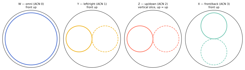
- W is an omni: the sound pressure at the listening point, direction-blind. Every source in the scene is in W at full level, wherever it is. If you keep only W, you have a correct mono mix — worth remembering when a client asks for the mono version.
- Y is a figure-8 aimed left–right: positive lobe left, negative lobe right. A source on the left appears in Y in phase with W; a source on the right appears polarity-flipped; a source dead ahead doesn't appear in Y at all.
- Z is the same figure-8 aimed up–down.
- X is the same figure-8 aimed front–back.
If you have ever set up a mid-side recording — a mid mic plus a sideways figure-8, matrixed into stereo width later — you already own the key intuition: B-format is mid-side, completed. M/S captures "the sound, plus how left-or-right it is." W/X/Y/Z captures "the sound, plus how left-or-right and front-or-back and up-or-down it is." Everything else about Ambisonics is this idea, refined.
Encoding is just gains
Now reread what ambitap.encode~ did in Chapter 3, in these terms. To
place a mono source in a direction, the encoder asks: what would each of
these coincident microphones pick up from a source over there? — and the
answer, per channel, is just a number. A source dead ahead: W gets 1, X
gets 1, Y and Z get 0. A source hard left: W gets 1, Y gets 1, X and Z get
0. A source up-front-left: some spread of positive fractions. Encoding a
source is multiplying one signal by one gain per channel — which you
verified with your own eyes on the mc.meter~ in Chapter 3, watching the
gains redistribute as the dial turned.
That's also why summing two encoded buses (Chapter 4) is legitimate mixing: each channel of the sum is exactly what that virtual microphone would have picked up with both sources playing. The bus doesn't store sources; it stores what the microphones hear, and microphones hear everything at once.
Higher orders: sharper microphones
Four coincident patterns can only distinguish direction so finely — you
felt that as first-order blur in Chapter 3's polar figure. The fix is
more patterns with more lobes. Second order adds five channels whose
shapes are cloverleaf-like, four-lobed patterns; third order adds seven
more, finer still. Each new order family adds 2n+1 channels, which is
why a full set to order N is (N+1)² — 4, 9, 16, 25, 36…
These higher patterns stop resembling anything in a mic catalogue, but their job doesn't change: each is one more coincident pickup pattern, one more independent measurement of the directional field, letting the scene distinguish directions the lower orders confuse. More measurements, sharper picture — precisely quantified in the next chapter.
For the curious. The patterns are the real spherical harmonics Ynm(θ, φ) — the natural basis for functions on a sphere, as sines and cosines are for functions of time. "Order" n is the polar degree; within an order, m runs −n…+n, giving the 2n+1 members. The encoder's gain for channel (n, m) is literally the value of Ynm evaluated at the source direction. The book's figures compute these through the library's
evaluate_sh— which is cross-checked against SciPy, spaudiopy, and pyshtools to float precision (docs/COMPARISON.md) — and Appendix D points to Zotter & Frank's open-access textbook for the derivations.
The two pieces of housekeeping
A basis is only usable if everyone agrees how to file it. Two conventions pin down the bookkeeping, and AmbiTap follows the modern standard (AmbiX) for both:
Channel order — ACN ("Ambisonic Channel Number"). Channels are indexed
acn = n(n+1) + m: W is 0; then Y, Z, X are 1, 2, 3; then the five
second-order channels 4–8, and so on. Note the first-order order: Y
before Z before X — not the historical "XYZ" — a fact that will matter
in Chapter 8, when we meet files that filed things differently.
Level scaling — SN3D. Each pattern needs a reference level. SN3D
scales so that no channel's gain ever exceeds W's: a unit source dead
ahead puts 1.0 in W and 1.0 in X, and anything higher-order lands at 1.0
or below. The practical consequences: your mc.meter~ never shows a
higher channel hotter than W for a single source, and W alone remains a
correctly-scaled mono mix.
You never chose these conventions in Part I, and mixing entirely inside AmbiTap you never need to — every object speaks AmbiX. The moment a file, a plugin, or a 2009 sample library enters the picture, conventions become the difference between a soundfield and soup. That's Chapter 8. First: what does order actually buy, in numbers you can plan a project with?