Two ears, infinite directions
Before you buy a single plugin or patch a single object, notice what you already own: the most sophisticated spatial audio system ever built. Two pressure sensors, one head between them, and a brain that turns their tiny disagreements into a continuous, three-dimensional map of everything sounding around you.
Every technique in this book — ambisonic encoding, decoder matrices, HRTF convolution, crosstalk cancellation — is in the business of manufacturing the input signals that system expects. So the right place to start is not with Ambisonics at all. It's with the question the rest of the book keeps answering: what do your ears actually measure?
The three measurements
Your auditory system localizes sound with three families of cues, and it helps to know all three by name, because every spatial audio tool is a machine for forging some subset of them.
Time. (ITD — interaural time difference.) A sound from your left reaches your left ear first. The head is roughly 17 cm wide, sound covers that in about half a millisecond, so the arrival-time difference between your ears ranges from zero (dead ahead or behind) to roughly 0.6–0.7 ms (hard left or right). Half a millisecond is nothing — a single video frame lasts sixty times longer — yet your brainstem resolves differences of ten microseconds. ITD dominates localization at low frequencies, below about 1.5 kHz, where the wavelength is long enough for timing comparisons between the ears to be unambiguous.
Level. (ILD — interaural level difference.) Your head is an obstacle. At high frequencies — wavelengths small compared to the head — it casts an acoustic shadow, so a sound from the left arrives at the right ear not just later but quieter, by up to 20 dB and more in the top octaves. At low frequencies the wave diffracts around the head almost unbothered and the level difference nearly vanishes. This division of labor — timing below ~1.5 kHz, shadow above — is the duplex theory, and it's over a century old.
Spectrum. Time and level differences share a blind spot: they're (nearly) identical for every point on a cone extending sideways from your ear — the cone of confusion. A source directly ahead, directly behind, and directly above can produce almost the same ITD and ILD (all ≈ zero). What breaks the tie is your outer ear. The pinna's folds reflect and resonate differently depending on the direction of arrival, notching and boosting the spectrum above ~4 kHz in a direction-dependent pattern your brain has spent your whole life learning. Elevation perception and front/back discrimination live almost entirely in these spectral fingerprints — which is why they're fragile, personal, and the hardest thing for any playback system to reproduce.
The figure below shows the first two cues, measured, not sketched: the interaural time and level differences of the KEMAR mannequin head — the standard measurement dummy whose ears this book's binaural renderer uses — as a source circles the horizontal plane.
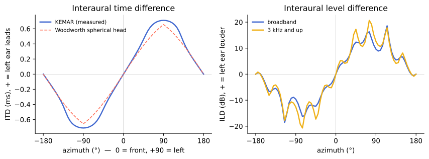
Two things worth noticing. The ITD curve is smooth, bounded, and maxes out around ±0.7 ms exactly as head geometry predicts. The ILD curve is larger, lumpier, and frequency-dependent — that's diffraction around an actual head, with actual ears attached, and its lumps are information, not noise.
For the curious. The duplex theory is Lord Rayleigh (1907); the modern, encyclopedic treatment of everything in this chapter is Blauert's Spatial Hearing. A convenient geometric approximation for ITD is Woodworth's formula, ITD ≈ (a/c)(θ + sin θ) for head radius a and sound speed c — the library's test notebooks check the embedded KEMAR data against it, and you can rerun that check yourself (
notebooks/hrtf_analysis.ipynbin the AmbiTap repository).
And one more cue that isn't a cue: movement. When time, level, and spectrum still leave ambiguity, you turn your head — a few degrees is enough — and watch how the cues change. Front/back confusions collapse instantly. Keep this in your pocket: it is the entire reason head tracking matters, and the reason Chapter 4 exists.
The experiment stereo fails
You don't need any of this book's tools yet. Build the classic MSP patch — a noise burst panned between two speakers or headphone channels:
[noise~] → [pan2 ...] → [dac~ 1 2] (any equal-power pan will do)
Sweep the pan and listen. Something does move. Now interrogate it:
- Where is "behind you"? Try to pan the noise behind your head. There is no knob for that. The image lives on a line between the speakers (or, on headphones, on a line through your skull — more on that in a moment).
- Where is "up"? Same problem. One axis was never captured.
- If you're on loudspeakers: move. Stand up, step a meter to the left, sweep the pan again. The image warps toward the nearer speaker and, from close enough to either one, collapses into it entirely.
What stereo panning actually is
Stereo panning is one trick performed well: play the same signal from two loudspeakers at different levels, and a listener seated exactly on the centerline hears a single phantom image somewhere between them. The pan pot moves the image by trading level between the channels — usually along an equal-power law so the loudness stays constant as it moves:
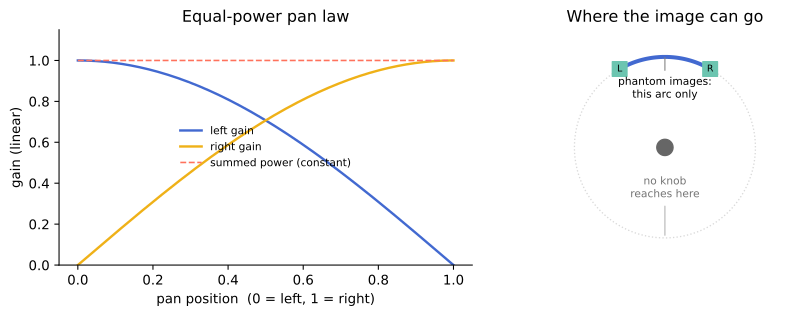
It's worth being precise about why this works, because the mechanism is sneakier than "the louder side wins." Both speakers reach both of your ears. At low frequencies, the two arrivals sum at each eardrum, and the level imbalance between the speakers converts into a timing shift of the summed waveform — fake ITD, synthesized out of pure level difference. The trick is genuinely clever. It is also narrow:
- It only works between the speakers — a ±30° window in front of you.
- It only works at one listening position. Off the centerline, the nearer speaker's earlier arrival dominates (precedence), and the image slides into it.
- It produces no elevation cues and no rear cues — nothing touches the pinna-spectrum channel, and nothing can place energy behind you.
- On headphones, with no crosstalk between channels at all, the level trick stops producing spatial impressions of an external world: images form on the axis between your ears, inside your head. Externalization — the difference between "sound to my left" and "sound in my left ear" — requires the full cue set, which plain level panning never forges.
None of this is a defect. Stereo is a 1930s-vintage compression scheme for space, brilliant within its window, and a century of great records testifies to it. But see it for what it is: a picture of a soundfield, painted on a narrow strip of wall, for a viewer nailed to one spot on the floor.
The point
Localization runs on ITD, ILD, and spectral cues — plus head movement to resolve ties. Stereo forges a sliver of that cue-space. Everything that follows in this book is a machine for forging more of it, more honestly:
- Ambisonic decoding (Chapters 5, 12) arranges many loudspeakers so the cues reconstruct over a listening area instead of a point.
- Binaural rendering (Chapters 3, 13) synthesizes the exact ear-entrance signals — all three cue families — for headphones.
- Head tracking (Chapters 4, 13) keeps the cues consistent when you move, which is the difference between a picture of space and a place.
- Crosstalk cancellation (Chapter 16) fights the physics of two speakers to deliver binaural signals through the air.
First, though, we need a language for storing a soundfield so that any of those machines can render it. That language question — and its three very different answers — is the next chapter.